Contact mechanics

Scientists, mathematicians and engineers have been studying the process for over a hundred years [11] [28]. For a wheel on a loaded freight wagon, the mean pressure within the contact patch is roughly 10 000 atmospheres: higher than the yield point of steel. Under these conditions, some of the metal below the rail surface will soften and flow like toothpaste. Fortunately, for reasons that we’ll go into later, the rail doesn’t collapse, although the repeated application of wheel loads does change the crystal structure of the material. Another curious feature of wheel-to-rail contact is that different processes can take place within the contact patch at the same time. In one sector, the surfaces grip each other tightly while in another, they slip.

What contact mechanics is about

Processes of this kind are studied under the general heading of contact mechanics. As you might imagine, contact mechanics is concerned with what happens when two solid objects are pressed together. We focus attention on the surface layers, and try to predict the stresses near the surface and how the two bodies deform. There are many situations where such knowledge is useful. For example, the components of a domestic washing machine are shaped on a factory production line using industrial tools such as punches and dies that impose high local stresses on the surface material. And almost all finished products are built up from components joined in compression, or moving parts such as ball bearings that slide or roll over one another. We want to know how the materials will behave, whether they will keep their shape, and in the case of moving parts, how quickly they will wear out.

Our modern understanding of contact processes is based on a theory that came from an unlikely source: a twenty-four year old physics research assistant at the University of Berlin. In 1870, Heinrich Hertz was investigating optical phenomena. If two glass lenses with slightly different surface radii touch one another as shown in figure 1, there will be a narrow gap around the point of contact where the light waves can produce interference fringes. Hertz was interested to see how the gap changed owing to minute levels of deformation in the glass when the lenses were squeezed together, and he devised an elegant theory to predict the deformation. It has since found applications in many branches of engineering.

Figure 1

The Hertz model

Hertz was originally interested in contact between spherical surfaces, but he was able to generalise his results to ellipsoidal (egg-shaped) surfaces each of which can be regarded as a sphere that is stretched in a particular direction (figure 2). Hertz showed that the contact area was elliptical, and worked out how the contact pressure varied from place to place within this ellipse. Starting from simple assumptions, he produced formulae for the localised stresses and also for the degree of deformation. Both can be expressed as a function of the applied load, the geometrical curvatures of the two surfaces, and the modulus of elasticity for the material from which each body is made.

Figure 2

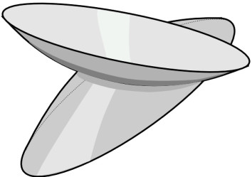
Figure 3

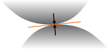
Hertzian contact theory, as it is known today, applies only to elastic bodies in non-conformal contact. To understand what is meant by ‘non-conformal’ it helps to imagine the contact process as a gradual one, starting with the two bodies separated by a small gap. Then we reduce the gap slowly until the surfaces touch. They have different profiles so that when they first touch, they do so at a single point or along a single line. They mustn’t meet over a finite area, as they would if, for example, if you laid a book on your desk or pressed a rolling pin into a lump of dough.

This greatly simplifies the geometry. We’ll leave the question of line contact until later, and for now, imagine a plane drawn through the contact point that is tangential to both surfaces (figure 3). We call this the contact plane, and it provides a useful frame of reference. To describe the shapes of the two bodies, all we need to know is the curvature of each body in the region of the contact area, defined by two curvature values at right angles to one another in the \(x\) and \(y\) directions located in the contact plane. Then to a first approximation, the distance \(z_{1}\) between the first body and the contact plane, and the distance \(z_{2}\) between the surface of the second body and the contact plane, both increase as the square of distance from the contact centre. This condition can be expressed mathematically [2] in the form:

where \(A_{1}\), \(A_{2}\), \(B_{1}\) and \(B_{2}\) are constant coefficients linked to the curvatures.

When a compressive force is applied that squeezes the two bodies together, the contact point becomes a finite area, but the area is small in relation to the sizes of the bodies concerned. A small contact area means that the stresses are quite concentrated and their values can be quantified independently of those in the rest of the body, which are small by comparison [12] [25]. In practice, two bodies fulfil these conditions if they both have a smooth surface and a large radius of curvature compared to the size of the contact area. This means that the bodies can be treated as though they extended indefinitely into three-dimensional space.

There are other limitations. The theory depends on there being no tensile forces and no tangential or shear forces between the objects concerned, in other words, the only pressure allowed is ‘normal pressure’ at right angles to the contact surfaces, with no friction. This might apply if the surfaces were separated by a liquid film as for example in the case of gear teeth in a well-lubricated gearbox, but it doesn’t normally apply to a wheel rolling on a railway track, where the contact force has both normal and shear force components. The presence of a shear force, as occurs between a wheel and the rail surface when a train driver applies the brakes, changes the stress pattern. So does the fact that the surfaces are rolling over one another. It was not until about 50 years ago that a satisfactory model emerged. It turned out to have far-reaching consequences, because it helped to explain why railway vehicles became unstable at high speeds, a problem that had dogged railways almost since the steam engine was invented. In what follows, we will begin by treating the wheel as stationary with no shear forces, and move on to rolling contact later.

Static contact

In practice, one can’t observe the contact patch directly, but from the limited data available [23] it appears to be roughly circular with an area of about one square centimetre, about the size of a human fingernail. As we’ll see later, given a rail surface that is curved in cross-section this is what Hertzian theory leads one to expect. However, one might equally well imagine that the rail surface wears flat, so the process more resembles a cylinder rolling on a table top [7]. In this model, the initial contact takes place along a straight line rather than a single point, and when pressure is applied, the line becomes a rectangular strip (figure 4). While the contact pressure can vary in the x-direction from the leading edge to the trailing edge, the profile is assumed to be uniform in the \(y\)-direction from one side of the railhead to the other. But why switch to a less realistic model? The mathematics follows Hertzian principles but the formulae turn out to be simpler, and although the results don’t quite match with reality they throw light on what would otherwise be a tricky subject.

Figure 4

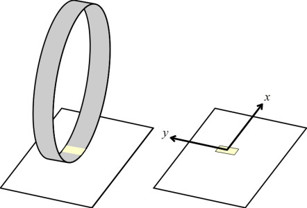
Figure 5

Cylindrical surface model

We’ll follow the exposition that appears in [14] and [26] using a slightly modified notation. According to principles first laid down by Hertz in 1882, the value of the normal contact pressure at a point \(x\) measured from the centre of the contact area in the direction at right angles to the axis of the cylinder is given by:

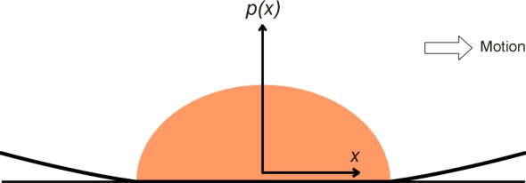
We assume that a stationary railway wheel generates a pressure distribution similar to that of the cylinder, and that the shape of the curve doesn’t change when the wheel starts to move. Suppose the length of the contact patch measured parallel to the direction of motion is \(2a\), and its width is \(2b\). Denote the tread radius by \(r\) and assume the wheel is carrying a load \(P\). As shown in figure 5, the pressure rises from zero at the leading edge of the contact patch to a maximum in the centre, and falls to zero at the trailing edge. The curve is semi-elliptical in shape, and the peak value \(p_{0}\) is given by:

The dimension \(a\) is related to \(P\) via:

where \(E^{*}\) is the contact modulus given by

The quantities \(\nu_{1}\) and \(\nu_{2}\) are the values of Poisson’s ratio for the two materials, while \(E_{1}\) and \(E_{2}\) are the respective Young’s moduli. If similar types of steel are used for the wheel and rail with

then equation (5) becomes

If we substitute for \(a\) in eq (3) using eq (4) we get

We now know the peak vertical pressure: it occurs at the rail surface along a line drawn transversely across the rail head bisecting the contact patch. But normal pressure is neither the only stress nor even the most important stress that the railhead must withstand. At any given point beneath the surface, the stress can be resolved into three components, each acting in one of the three directions \(x\), \(y\), \(z\) (figure 6). In addition there are shear stresses acting in the three planes \(xy\), \(xz\) and \(yz\). It turns out that while the vertical stress diminishes rapidly with depth, the shear stress starts at zero and rises to a maximum a short distance below the surface (figure 7). It can be shown that the maximum is equal \(0.30 p_{0}\) and it occurs at a depth equal to \(0.78 a\) [14]. In practice, this maximum arises only in the lateral \(yz\) plane [10].

Figure 6

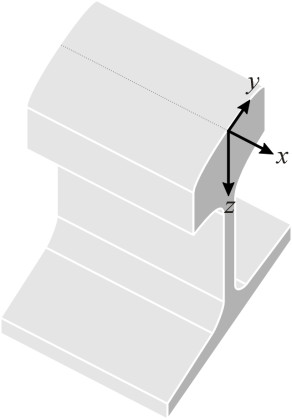
Figure 7

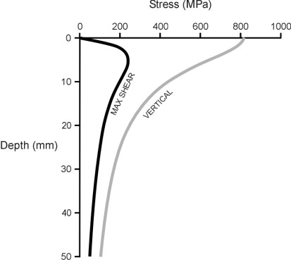
Let’s put some numbers into equations equation 3 and equation 4 by way of illustration. For a wheel of radius 0.45 m carrying a load of 10 tonnes on a rail for which the Young’s modulus is 210 GPa and Poisson’s ratio 0.3, if we assume a typical contact patch width of 12 mm, the length \(2a\) of the contact patch comes to a little under 13 mm and the peak compressive stress 817 MPa. Also, one can show that the maximum shear stress in the rail head is about 245 MPa and it occurs at a depth of about 5 mm. Generally speaking it is the shear stress rather than the compressive stress that makes a metal such as steel deform: yielding is a shear phenomenon. This explains why the surface of a rail will often flake away indicating a crack whose origin lies a few millimetres below the surface [10].

Ellipsoid surface model

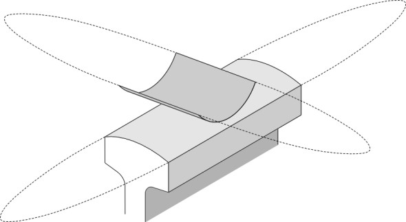
This simple picture of a cylinder resting on a flat surface has turned out to be very useful for the railway engineer [9] because it helps to explain the behaviour of a rolling wheel. But before pressing on, let’s check how far the results depart from reality, given that a rail, at least when it is new, will be curved in cross-section. Effectively, we have two ellipsoidal surfaces in contact, with the rail stretched indefinitely in the longitudinal direction so its radius in the \(xz\) plane is infinite (figure 8). The contact patch is elliptical, and an analysis based on Hertzian principles leads to a different set of formulae for the contact patch dimensions and stresses within the rail head (incidentally, the frame of reference [\(x\), \(y\), \(z\)] is aligned with the contact plane between wheel and rail at the centre of the contact patch, so \(z\) is not quite vertical, rather inclined at an angle \(\gamma\) to the track frame of reference where \(\gamma\) is the cone angle, but this doesn’t greatly affect the outcome).

Figure 8

Using these formulae one can re-evaluate the example we looked at earlier, but now with a curved rail surface, and in addition, we’ll assume that rather than being conical, the wheel tread is worn into a curved profile in cross-section. We’ll take the radius of this curve as -1000 mm (negative because it is concave), and the radius of the rail in cross-section as 250 mm. The formulae are complicated and they are not reproduced here, but you can find them for example in [13]. It helps to set them up in a spreadsheet. For the above example the longitudinal dimension \(2a\) of the contact patch comes to just under 14 mm, the width \(2b\)a little over 11 mm, and the peak normal pressure at the centre of the contact patch 1.2 GPa. Compared with the earlier model, the contact patch has similar overall dimensions but the peak pressure is about half as much again.

Rolling contact

So far we have been following in the footsteps of Heinrich Hertz, who was concerned only with normal contact pressure between two surfaces: contact with no friction and therefore no shear stresses between them. But these conditions don’t apply to a railway wheel, for two reasons. First, the wheel is rotating so each part of the tread repeatedly enters the contact patch and exits at the trailing edge. This doesn’t affect the normal pressure distribution, which remains broadly the same as for a stationary wheel, but as will be explained shortly, the intermittent loading and relaxation process allows relative movement between the wheel and rail. Secondly, shear stresses arise whenever the driver applies the brakes - or in the case of a powered axle, whenever the motor applies a torque in order to push the vehicle along. So we now have both a normal force \(P\) and a shear force \(Q\). One of the curious things about the railway contact patch is that when a driving force or a braking force is applied to the wheel, even a very small force, in one or more parts of the contact patch the shear stresses will exceed the frictional resistance and relative slip will occur. This is doubly curious insofar as the wheel are rail remain firmly stuck to one another over the rest of the contact patch. Slip and stick occur simultaneously in regions only millimetres apart.

Stick and slip

It’s helpful to refer to whatever slipping goes on inside the contact area as ‘micro-slip’ to distinguish it from what happens when the wheel slides bodily along the track. Micro-slip is a tiny movement that occurs locally in places where the applied shear stress exceeds the frictional capacity of the two surfaces. How is it possible for one part of the wheel tread within the contact area to slip over the rail while in another part, it remains firmly locked?

Figure 9

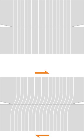
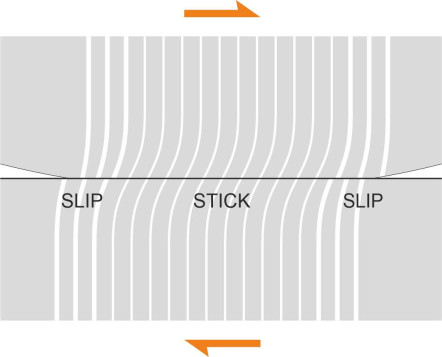
To understand how and where this happens, we’ll start with a simple case and assume that the wheel is not actually moving – although it’s being pushed forward to the right as shown in figure 9. This can happen, for example, when a vehicle is parked on a gradient with the brakes holding the wheel so it ‘feels’ a shear force \(Q\) that prevents the wheel from sliding downhill. The shear force is distributed across the contact area as a shear stress, and both the wheel and the rail surfaces deform. We want to know how this shear stress varies from the leading edge to the trailing edge, and at each point this depends on the normal contact stress acting at right-angles to the rail surface. This arises from the weight of vehicle pressing down on the rail, and like the shear force it is distributed along the contact area.

Now, as a first guess, we might suppose that the shear stress is uniform along the whole length of the contact area, but here we run into a problem. Earlier in figure 2 we saw that the normal stress peaks at the centre and falls to zero at the front and rear. Since there’s no normal stress at the leading and trailing edge, there can be no friction and crucially, no shear stress to deform the surface of the wheel or rail. Here, the deformation is zero, so the wheel and rail surface both relax, slipping over one another as shown in figure 10. The amount of slippage is very small, but it’s physically significant. So how do we determine the shape and size of the ‘stick’ and ‘slip’ areas? The problem was first solved by Cattaneo using the guiding principle [15] [20] that all surface points within a stick region undergo the same tangential displacement. If the two bodies have the same elastic constants, the displacements are equal and opposite.

Figure 10

Let the shear force be large so that the wheel is just about to slide bodily along the rail. Here we have the maximum possible shear load that the system can sustain, with each segment of the contact patch generating a frictional resistance equal to the coefficient of friction \(\mu\) times the normal force carried by that segment. Since the normal stress follows the profile specified by equation 2, the shear stress profile, which we’ll denote by \(q'(x)\), must be [16]:

When we sum over the contact area as a whole, the total comes to \(\mu\) times the wheel load or \(\mu P\), as it would in any school lab experiment. Next, let us reduce the shear load somewhat. The contact area will still be saturated towards the leading edge and trailing edge but in between, in a region of length \(2c\) say, the stress will fall below the envelope specified in equation 9. To represent what happens in this central stick region we subtract a stress profile whose value is calculated exactly to equalise surface displacements over the distance \(-c \leq x \leq c\). This profile can be shown to take the form [16]:

The length \(2c\) of the central strip is determined via

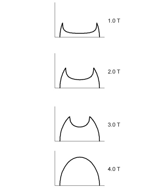
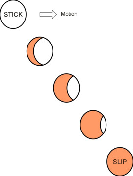
The resulting shear stress profile is shown in figure 11. Notice the characteristic dip in the centre. Finally, using these formulae we can reconstruct what happens if the shear force is applied gradually starting from zero: as shown in figure 12 slip begins at the edges and progresses towards the centre, while the central stick region shrinks until it disappears and full sliding occurs [17].

Figure 11

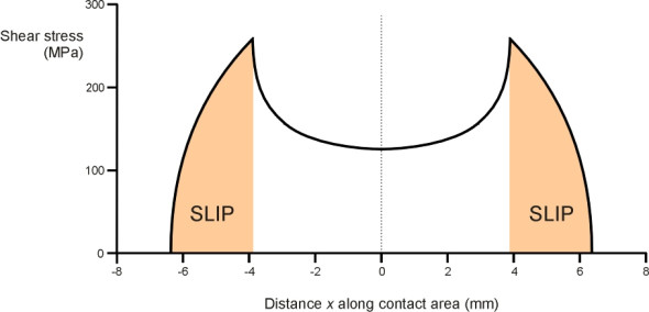
Figure 12

Shear stress in rolling contact

The picture changes when the wheel starts to roll. To see how, let us choose a small area of the tyre tread and follow its progress during a typical encounter with the rail surface (what applies to the wheel tread also applies to the rail surface, each element of which undergoes a similar loading and unloading cycle when the axle passes overhead). We are interested in the evolution of both the normal stress and the shear stress acting on this element as it passes through the contact area when the driver applies the brakes. Before the element arrives at the leading edge, both stresses are zero. When it enters the contact area, the normal pressure changes: as you might expect, it builds up to a peak in the centre of the contact area and then declines to zero at the trailing edge, and in the process, traces out a profile closely resembling that for the static case (for the purpose of analysis, it is usual to assume in fact that the two profiles are identical).

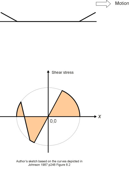
The evolution of the shear stress, however, is a different matter. When the wheel is stationary, there is slip at the leading edge, slip at the trailing edge, and stick in between, but the slip towards the leading edge cannot be sustained when the wheel rotates because it is in the ‘wrong’ direction. This involves some rather convoluted reasoning [5] that we won’t go into here. What matters is that the ‘stick’ region moves forwards to the leading edge, leaving a single slip region at the rear. It can be shown that this solution meets all the mathematical criteria and it seems to represent what happens in real life. So all we need to do is shift the component \(q''(x)\) in equation 11 forward by a distance \(d = a - c\) [19]. The new shear stress profile is shown in figure 13. This vital modification was first suggested by F N Carter in 1926 [8]. More recently, it has been possible to model the transition in detail, starting from Cattaneo’s solution for the stationary case and terminating in steady rolling according to Carter’s scenario. The transition takes place very quickly [22].

If you’ve managed to get this far, you’ll want to know what happens if we now put aside the cylindrical model and revert to a more realistic representation of the rail surface. Working at the Delft Institute of Technology in the Netherlands, Professor J J Kalker has developed simulation models that reproduce the rounded shape of the contact patch on a curved rail surface, built up as a series of longitudinal strips. In this model, when viewed in plan the slip-stick frontier looks like a moon quarter [21] as shown in figure 14. The precise shape depends on the shear force. If a train is coasting along with no brake force applied to the wheel, there is no slip and the frontier vanishes. But if the driver applies the brakes (we assume they are applied gradually), a slip area will appear at the trailing edge and the frontier will move forward until under maximum braking effort it covers the whole contact area (figure 15), at which point the wheel loses adhesion altogether and begins to slide along the rail surface [3].

Figure 13

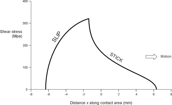
Figure 14

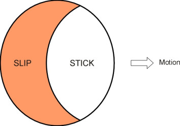
Figure 15

Free rolling

We have now looked at two cases: a stationary wheel, and a rolling wheel accompanied by a shear force of the kind that arises in traction or braking. To complete the picture, let us think about a wheel that is coasting, i.e., rolling freely with no longitudinal forces at all. Will there be any rolling resistance, and if so, how does it come about? As we have seen already in the case of the car tyre (Section C2019), rolling resistance can arise from frictional energy losses associated with micro-slip within the contact patch [27]. However, railway vehicles are puzzling because the wheel and the rail are made from similar materials, and if they have identical mechanical properties, symmetry tells us that without an externally applied shear force there can be no slippage and they behave as a single body [18]. Hence there can be no rolling resistance. The puzzle can be resolved in two ways. First, at a microscopic level the contact stresses don’t have the smooth profile that we have assumed so far. The surfaces are rough and contact takes place at local peaks that occupy a relatively small proportion of the contact area. Here, the contact stresses are well above the yield point of steel, which flows plastically and absorbs energy in the process.

Secondly, the physical constants or moduli that describe the elastic behaviour of the wheel material and the rail material are not quite identical. Using a combination of theory, simulation, and experiment, analysts have pieced together the stress profile that is likely to occur under these conditions [18]. The pattern as a whole can be described as S-shaped, with the shear stress acting outwards (away from the centre of the contact patch) on the more compliant material and inwards on the more rigid one, with a stress reversal in between. There is in addition a second stress reversal close to the trailing edge. Assuming that the wheel material is more compliant than the rail material, the resulting profile is reproduced in figure 16, which shows the shear stress on the wheel measured positive in the ‘ahead’ direction. It looks a little like the shear stress profile acting on a car tyre (see Figure 4 in Section C2015), but the mechanisms are different and the resemblance may be coincidental. In any case, the net force in the case of the railway wheel is miniscule by comparison: the rolling resistance of a steel wheel on a steel rail is almost too small to measure. In practice, most of the rolling resistance of a railway wheel arises from the intermittent impacts of the flange against the inside face of the rail that occur when the vehicle lurches from side to side, or presses against the outer rail on a curve.

Figure 16

Creep

It’s a useful trick to imagine yourself travelling along with the wheel. You can look down at the contact area and watch the wheel tread flowing like a continuous stream through the contact patch, and likewise the rail itself. Surprisingly, when the wheel is subject to a shear force, the two streams don’t flow at exactly the same speed. Even though they grip each other firmly as they travel through the ‘stick’ area of the contact patch, if there is a ‘slip’ region each element of the tread will emerge slightly earlier or later than its partner in the rail head. The result is something called creep, a continuous relative movement between the wheel tread and the rail surface.

Figure 17

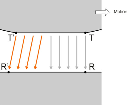
Let’s assume that the vehicle is rolling steadily along when the driver applies the brakes. Choose a tread element just as it enters the contact patch at T as shown in figure 17. We’ll track its progress together with the corresponding rail element that enters the contact area at R at the same moment. The tread element and the rail element progress through the leading part of the contact patch locked together. When they reach the slip-stick frontier, the tread element will slip forward relative to the rail element and emerge from the trailing edge slightly later. Hence the wheel revolves more slowly than it would do if the vehicle were rolling freely without any braking force. Similarly with a driven wheel except that the position is reversed: the tread element emerges first and the wheel rotates faster. The disparity is usually expressed as a creep rate\(\; \upsilon_{x}\), this being the relative speed \(\dot x\) in the forward direction expressed as a proportion of the rolling speed \(V\) so that

The larger the shear force, the greater the creep rate, so that when the shear force reaches the maximum value that the contact area can sustain with the ‘stick’ area on the point of vanishing altogether, the quantity \(\upsilon_{x}\) approaches a value of 0.01 to 0.02 [24]. In other words, the speed difference can reach a value between 1% and 2%.

The speed difference may be small, but it allows a degree of flexibility between the wheel and the rail which in turn leads to a particular kind of instability known as hunting. It was in 1916 that the mathematician and engineer F W Carter identified the underlying cause of hunting, and later he published a mathematical formula describing the key relationship between shear force and creep [6]. As we shall describe later in Section R1717, the relationship is approximately a straight line, and the slope of this straight line can be interpreted as a ‘stiffness’ that controls the oscillating motion. His formula was used until the 1960s. However, it was derived from a two-dimensional model of the wheel rolling like a cylinder on a flat plane, and it was not until 1967 that J J Kalker succeeded in developing more accurate stiffness coefficients based on a three-dimensional representation of the contact area, the results being confirmed by experiment [1] [4]. In addition to longitudinal creep, there are coefficients for lateral creep because the wheel can move from side to side across the top of the rail head as well, giving rise to a lateral creep rate \(\upsilon_{y}\).

Conclusion

If you want to make a wheel that can carry a vehicle across a prepared surface of some kind you can choose from several possibilities. The pneumatic tyre on a concrete road represents one possibility in which the load is spread over a relatively large area. The steel wheel and the steel rail represent the opposite extreme: the load is concentrated within a tiny contact area so as to minimise rolling resistance. Although the contact area is small, the stresses are not uniform inside the boundary and when the wheel is subject to a shear load during braking or acceleration, one observes two distinct areas. There is locked contact in the leading portion and micro-slip in the trailing portion: as with a pneumatic tyre, the slip area is always at the rear regardless of whether the wheel is braked or driven. Moreover the slip allows the tread and the rail to flow at slightly different speeds through the contact area even though they are firmly locked together in the leading portion. The contact is slightly elastic: it allows a degree of relative movement that wouldn’t occur if the wheel were a toothed pinion rolling along a toothed rack. In a later Section (R0418) we’ll see how this elasticity can make the vehicle unstable. But first, we’ll look more closely at the friction forces involved.