F.0515
Drift
When you are walking in the countryside, you scan the ground ahead, choose what looks like a suitable path and follow it, confident that the ground won’t shift under your feet. But when sailing in a boat, you have to watch out, because a current may carry you away from your destination. Similarly, if you take to the air, a crosswind may blow your aircraft off-course. The problem is that your vehicle is immersed in a fluid medium, and the fluid (air or water as the case may be) is itself moving, not necessarily in the direction you want to go. Sailors and aircraft pilots are trained to recognise the problem and do something about it: it’s one of many problems that together make up the wider subject of navigation. In this Section, we’ll concentrate on a specific issue: how to compensate for the drift by pointing the vehicle in the most appropriate direction. The geometry is not as simple as it looks. Analysis will reveal the best course to steer in a cross-current (easy), and what will happen if you just point the vehicle at the target (more difficult). There’s also the question of how much longer it will take to get there in a strong current, and indeed whether you’ll get there at all.
Figure 1
A special case
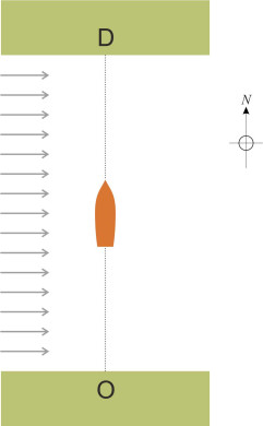
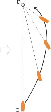
Suppose you are trying to cross a river. You start from the point labelled ‘O’ in figure 1, and your destination is the nearest point ‘D’ on the opposite side. The banks of the river are parallel and the water is moving everywhere at the same velocity at right-angles to your intended path. It’s a foggy day and you can’t see the opposite bank. Well, you probably ought not to be sailing at all in such conditions, but since you know the compass heading in which your destination lies (it’s due north), let’s see what happens if you set out in that direction and maintain the same compass heading throughout.
Figure 2
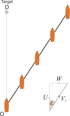
No correction
The path that your boat will follow – its ground track – will be different from its path through the water, and not at all the one you intended. Suppose that the speed of your boat relative to the water is \(U\), and that the speed of the water current is \(W\) relative to the earth. Then figure 2 shows that your ground speed \(V_1\) relative to the earth as the fixed frame of reference will be greater than your speed \(U\) relative to the water:
(1)
\[\begin{equation} V_{1} \quad = \quad \sqrt{U^{2} + W^{2}} \end{equation}\]You will follow a path lying at an angle \(\varepsilon\) downstream of the line OD given by
(2)
\[\begin{equation} \varepsilon \quad = \quad \arctan \left( \frac{W}{U} \right) \end{equation}\]Consequently, you’ll drift off-course and miss the target. So it might be better to wait until the weather has cleared, and try again using a different tactic.
Point and pursue
If you can see your destination, a more sensible tactic is to adjust your course continuously so the boat points directly at D throughout: that way, you can’t miss the target, or so it would appear. Forget about the ground track for a while and think about your path relative to the water around you as the frame of reference. Because the current is carrying you sideways, your destination D will appear to move at constant speed across your field of vision. As you keep turning the boat to point at D, your path through the water will no longer follow a straight line, but rather a curve of pursuit, one of a geometrical family of curves known to scientists and engineers for over 250 years. The curve was formulated in 1732 by the French mathematician Pierre Bouguer (1698-1758) to describe how a predator might chase its prey, such as a fox chasing a rabbit. The rabbit is running in a straight line at constant speed across the fox’s path, and the fox runs towards it at constant speed while continuously changing its heading (figure 3).
Figure 3
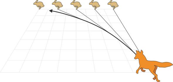
Figure 4
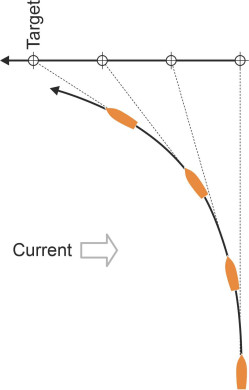
The curve can also be applied to sailing in a cross-current or flying in a crosswind: your path through the water curves as if you were ‘chasing’ your destination in the same way that the fox chases the rabbit (figure 4). But it doesn’t tell us the path of your vehicle relative to the earth as frame of reference, which will appear as shown diagrammatically in figure 5, and it’s not a simple matter to deduce the latter from the former.
Figure 5
To find the equation for this curve, imagine that the earth is marked out in Cartesian coordinates. Your journey starts at the origin (0,0), and you travel at constant speed \(U\) through the water. Your destination lies on the \(y\)-axis at (0,\(s\)). As before we’ll consider only the special case where the water is moving at constant speed \(W\) in the direction of the \(x\)-axis at right-angles to your initial course. Your path relative to the earth (ground track) will then satisfy the equation:
(3)
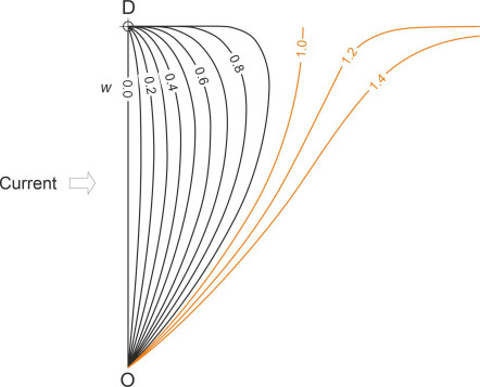
\[\begin{equation} x \quad = \quad \frac{1}{2} s \left[ {{\left( 1-\frac{y}{s} \right)}^{1-w}}\ -\ {{\left( 1-\frac{y}{s} \right)}^{1+w}} \right] \end{equation}\]where \(w\) is the ratio \(W/U\) of the speed of the current to your speed through the water. The derivation of equation 3 is set out in the Appendix to this Section. It is based on the one that appears on the Maths Stack web site [1] but in a different notation. Some typical results are shown in figure 6. Each curve represents your ground track given a particular current velocity. You can see that when the current moves slowly (\(w\) is small) your ground track is nearly a straight line, and that it deviates increasingly as \(w\) increases. The red curves correspond to the case where \(w \geq 1\): the current is moving faster than the speed of your vehicle through the water, and even though your boat remains pointing towards your destination throughout, you will not actually reach it.
Figure 6
Heading correction
The problem with the ‘point and pursue’ strategy is that your boat doesn’t travel in a straight line relative to the water, so you will waste fuel and your journey will take longer than it ought. So let’s try again. This time, we’ll compensate for drift by pointing the vehicle at an angle \(\psi\) upstream of D, an angle we’ll call the heading correction. The aim is to minimise the distance you will travel through the water. You might guess that if you chose a heading correction equal and opposite to the angle of drift \(\varepsilon\) in the earlier example, the two would cancel out and you would arrive exactly on target.
Figure 7
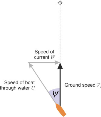
This is approximately true if the speed of the current is small relative to the vehicle speed, and in fact a standard procedure used by the pilots of light aircraft is based on the assumption that they are numerically equal [3]. However, this is not the case. From equation 2 we see that the drift angle equals \(\arctan{ \left( W/U \right) }\), whereas the correct heading as obtained from the vector diagram in figure 7 is given by:
(4)
\[\begin{equation} \psi \quad = \quad \arcsin \left( \frac{W}{U} \right) \end{equation}\]which is slightly larger than \(\varepsilon\). At this heading, your ground speed \(V_2\) will be
(5)
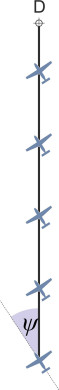
\[\begin{equation} V_{2} \quad = \quad \sqrt{U^{2} - W^{2}} \end{equation}\]Note that this is less than your speed relative to the water. The cross-current will slow your boat down so the journey takes longer and you will need more fuel than you would if there were no current at all. If you hadn’t thought about it before, you might not have expected that a cross-current at right-angles could slow a vehicle down in this way, but it happens to all craft immersed in a fluid that itself is free to move: ships, air cushion vehicles and aircraft alike. It happens because the vehicle must turn into the cross-current slightly and travel a greater distance through the air or water to maintain the required ground track. But as figure 8 shows, at least with the appropriate heading correction, the vehicle will travel in a straight line and arrive at its destination in the shortest possible time. Remember that this is a special case, and we must now consider what happens if the current flows in some other direction.
Figure 8
General case
Let’s look at the general case where the angle \(\phi\) between the line OD and the current vector is no longer fixed at \(90^{\circ}\) . From now on we’ll picture the vehicle as an aircraft rather than a boat, although the same principles apply. We’ll assume the wind is coming from the left: the case where it is coming from your right can be treated as the mirror image. The aim is to work out a heading correction that takes the aircraft in a straight line to your destination, i.e., in the shortest possible time. Your target appears to be moving from right to left across your field of vision, and rather than aiming at it directly, you aim for the place where the target will be when your aircraft crosses its path. It’s a more sophisticated approach, used not only by humans but also by dogs, fish, and spiders when chasing their prey [2]. The spiders, you’ll be relieved to hear, can’t do mathematics. Like other cunning predators, they use a simple algorithm that guarantees interception. Put yourself in the spider’s position. All you have to do is adjust your heading so the prey remains at the same bearing angle throughout. If it’s moving across your field of vision, say from right to left, you turn a little to the left and keep turning until the angle between your path and the target stabilises at a constant value - you’re not pointing at it, but ahead of it.
Here, we’ll tease out the maths. It is simplified if we fix the wind vector as our frame of reference and consider what happens to the aircraft when it points in one of many possible directions relative to the wind rather than the other way round. We can also reduce the number of variables by working in terms of the following dimensionless parameters:
(6)
\[\begin{equation} v \quad = \quad \frac{V}{U} \end{equation}\](7)
\[\begin{equation} w \quad = \quad \frac{W}{U} \end{equation}\]in which \(v\) is the dimensionless ground speed and \(w\) the dimensionless wind speed. A value of \(w\) greater than 1 signifies a fierce storm in which the air mass is moving faster than the aircraft can fly in a dead calm.
Moderate wind speeds
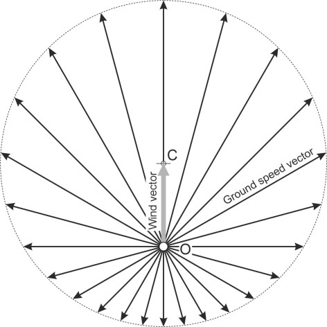
Normally, \(w\) will be very much less than 1. Figure 9 shows the wind vector \(w\) aligned with the vertical axis, rooted at the origin O and terminating at C. You can estimate the ground speed graphically for any particular direction of travel by drawing the ground vector as a straight line from O at an angle \(\phi\) to the wind vector and terminating at D where it intersects a unit circle centred on C. The ground speed and direction are then represented by the vector OD. The black arrows in figure 10 show graphically how the ground speed will vary as your aircraft attempts different ground track directions relative to the wind. As you might expect, travel is fastest when you fly in the same direction as the wind, with \(\phi = 0^{\circ}\) and \(v = 1+w\) (incidentally, commercial airline pilots don’t necessarily use a tail-wind to fly faster – they will often throttle back and fly more slowly to save fuel). By contrast, flying is slowest against a headwind, with \(\phi = 180^{\circ}\) and \(v = 1-w\). The ground speed will vary between these two extremes for other values of \(\phi\).
Figure 9
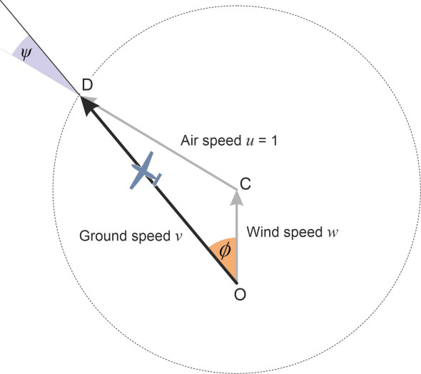
Figure 10
You can work out the numerical value of the ground speed by splitting the triangle OCD in figure 9 imto two smaller right-angled triangles. Without going into detail, the result is
(8)
\[\begin{equation} v \quad = \quad w \cos \phi \ + \ \sqrt{1-w^{2} \sin^{2} \phi } \end{equation}\]in which the second term on the right-hand side is evaluated as the positive square root. You can use a similar method, or alternatively, apply the sine rule to triangle OCD, to find the appropriate heading correction \(\psi\); as the pilot, you will need to steer at this heading to maintain the ground track OD that will take you straight to your destination. The result is given by
(9)
\[\begin{equation} \psi \quad = \quad \arcsin \left( w \sin \phi \right) \end{equation}\]
High wind speeds – will the plane get there at all?
Up to now we have assumed that the speed of the current is modest, so that we can expect to make progress in whatever direction we choose, against the current if necessary. This is almost always the case for aircraft (and for ships in an ocean current) but not necessarily for a hovercraft, which, assuming a maximum air speed of 120 km/h, may not be able to operate in severe wind conditions at all. From time to time, migrating birds, fish, and long-distance swimmers face a similar problem. Sticking with aircraft for the time being, the situation where \(w > 1\) is depicted graphically in figure 11. The range of possible ground directions is now limited, with the angle between the ground track and the wind vector confined to the range \(\pm \ \phi_m\), where \(\phi_m = \arcsin(1/\omega)\). It’s impossible to reach a destination outside this sector.
Figure 11
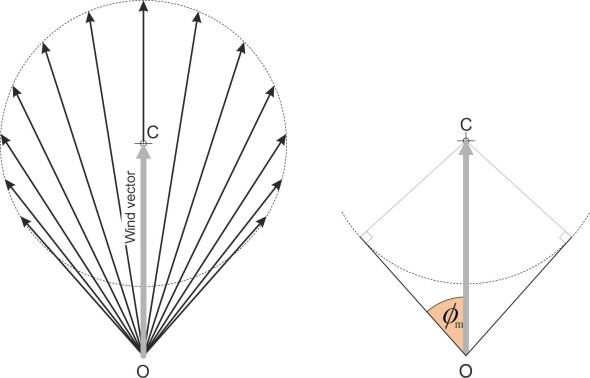
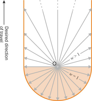
figure 12 depicts the influence of a strong wind in a different way. The grey arrows are wind vectors rooted at O. They represent critical wind conditions under which an aircraft can just make progress towards its destination. A wind vector that projects outside the red line will take the aircraft away from its destination. From the diagram you can see that if the wind is blowing in a favourable direction, an aircraft can reach its destination even if its air speed is low relative to the wind speed. However, it may not be able to make the return trip until the wind dies down!
Figure 12
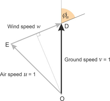
The neutral wind vector
We started with a specific problem, showing that a cross-current at right-angles to the intended ground track actually slows a boat down. This leads to an obvious question, which for the sake of argument we’ll phrase in terms of a moving aircraft. We can divide all possible wind directions into two sectors: those that assist the aircraft by speeding its journey towards its destination, and those that slow it down. At what angle does the wind have a neutral effect so that it neither helps nor hinders progress? In this case, we put \(v = u = 1\) and denote the specific wind angle that leads to this condition by \(\phi_n\). The geometry is shown in figure 13 (we assume that \(w < 2\) because a wind-neutral ground track does not exist for \(w \geq 2\)). The triangle OED is an isosceles triangle so that
(10)
\[\begin{equation} \cos \phi_{n} \quad = \quad \frac{\left( w/2 \right)}{1} \quad = \quad \frac{w}{2} \end{equation}\]therefore
(11)
\[\begin{equation} \phi_{n} \quad = \quad \arccos \left( \frac{w}{2} \right) \end{equation}\]You can see that if a wind-neutral vector exists, \(\phi_n\) is always less than \(90^{\circ}\), meaning that in the neutral case there must be a small velocity component in the direction of travel; in other words, the wind must be slightly ‘behind’ the vehicle.
Figure 13
Conclusion
This last result leads us to a curious conclusion. We have divided all the possible wind directions into two sectors, and the range of ‘favourable’ directions is smaller than the range of ‘unfavourable’ ones: the wind is more often a hindrance than a help. Other things being equal, this implies that on average world-wide, aircraft will reach their destinations more quickly on a calm day than they will on a windy one. And as the energy in the earth’s atmosphere continues to increase with global warming, we can expect to see more windy days and fewer calm ones, so that overall, air travel could become a little slower.
Appendix: Derivation of point-and-pursue curve
Figure 14
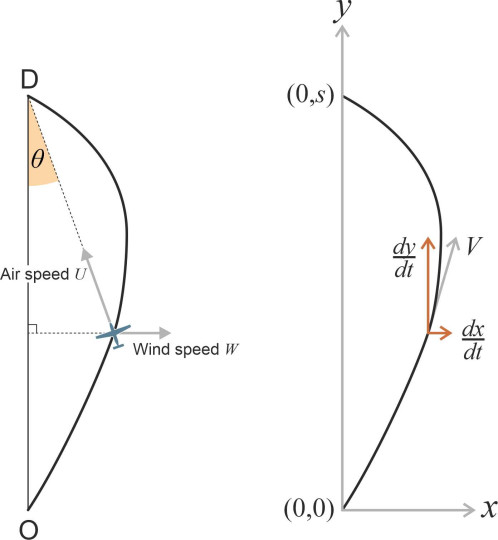
In figure 14, the \(x\), \(y\) plane represents the earth’s surface, with your trip starting at the origin O and finishing at your destination D on the \(y\)-axis. Denote time by \(t\). The wind is approaching from the left, parallel to the \(x\)-axis, at constant speed \(W\). Your aircraft travels with a constant speed \(U\) through the air mass, but its speed \(V\) relative to the earth varies from place to place along the journey. The curved line shows the path your aircraft will take if at each stage you keep the nose pointed directly at D throughout. We start by breaking down your ground speed into two separate components, one parallel to the \(x\)-axis and one parallel to the \(y\)-axis. We have
(12)
\[\begin{equation} \frac{dx}{dt} \quad = \quad W\ -\ U\sin \theta \quad = \quad W\ -\ Ux{\left[ x^{2} + (s-y)^{2} \right]}^{-\frac{1}{2}} \end{equation}\](13)
\[\begin{equation} \frac{dy}{dt} \quad = \quad U \cos \theta \quad = \quad U(s-y){\left[ x^{2} + {(s-y)}^{2} \right]}^{-\frac{1}{2}} \end{equation}\]By invoking the Chain Rule, we can combine these two into a single equation which after simplification becomes:
(14)
\[\begin{equation} \frac{dx}{dy} \quad = \quad \frac{W}{U} \frac{{\left[ x^{2} + {(s-y)}^{2} \right]}^{\frac{1}{2}}}{\left( s-y \right)}\ -\ \frac{x}{\left( s-y \right)} \end{equation}\]and after substituting \(w\) for \(W/U\), with a little rearrangement we get
(15)
\[\begin{equation} \frac{dx}{dy} \quad = \quad w \left[ 1 + \frac{x^2}{{\left( s-y \right)}^{2}} \right]^{\frac{1}{2}}\ -\ \frac{x}{\left( s-y \right)} \end{equation}\]Now we introduce a new variable
(16)
\[\begin{equation} \lambda \quad = \quad \frac{x}{s-y} \end{equation}\]so that
(17)
\[\begin{equation} x \quad = \quad \lambda \left( s-y \right) \end{equation}\]After differentiating both sides with respect to \(y\), equation 17 becomes
(18)
\[\begin{equation} \frac{dx}{dy} \quad = \quad \left( s-y \right) \frac{d\lambda }{dy}\ -\ \lambda \end{equation}\]We can now substitute the right-hand side of equation 18 for \(dx/dy\) and also \(\lambda\) for \(x/\left( s-y \right)\) in equation 15 to get
(19)
\[\begin{equation} (s-y) \frac{d\lambda }{dy}\ -\ \lambda \quad = \quad w{\left( 1 + {\lambda }^{2} \right)}^{\frac{1}{2}}\ -\ \lambda \end{equation}\]which after removing the term \(-\lambda\) from both sides can be written
(20)
\[\begin{equation} \frac{d\lambda }{\sqrt{1+\lambda^{2}}} \quad = \quad w \frac{dy}{\left( s-y \right)} \end{equation}\]We can integrate both sides of this equation (each side is a standard integral) to get
(21)
\[\begin{equation} {\sinh }^{-1} \lambda \quad = \quad -w \log_{e} \left(s-y \right)\ +\ C \end{equation}\]where \(C\) is a constant of integration which can be evaluated by noting that, at the origin, \(x = 0\), \(y = 0\) and therefore \(\lambda = 0\). Substituting these values in equation 21 we work out that
(22)
\[\begin{equation} C \quad = \quad w \log_{e} s \end{equation}\]so that equation 21 becomes
(23)
\[\begin{equation} \sinh^{-1} \lambda \quad = \quad - w \log_{e} \left( s-y \right)\ +\ w\log_{e} s \quad = \quad \log_{e} \left[ \left( \frac{s-y}{s} \right)^{-w} \right] \end{equation}\]which implies that
(24)
\[\begin{equation} \lambda \quad = \quad \sinh \left\{ \log_{e} \left[ \left( \frac{s-y}{s} \right)^{-w} \right] \right\} \end{equation}\]But by definition
(25)
\[\begin{equation} \sinh (z) \quad = \quad \frac{1}{2}\left( e^{z} - e^{-z} \right) \end{equation}\]so by expanding the right-hand side in this form, equation 25 becomes
(26)
\[\begin{equation} \lambda \quad = \quad \frac{1}{2} \left[ \left( \frac{s-y}{s} \right)^{-w} - \left( \frac{s-y}{s} \right)^{w} \right] \end{equation}\]and substituting back for \(\lambda\) via equation 16 this leads to the result
(27)
\[\begin{eqnarray} x \quad & = & \quad \frac{1}{2}\left( s-y \right) \left[ \left( \frac{s-y}{s} \right)^{-w} - \left( \frac{s-y}{s} \right)^{w} \right] \nonumber \\ & = & \quad \frac{1}{2} s \left[ \left( 1-\frac{y}{s} \right)^{1-w} - \left( 1-\frac{y}{s} \right)^{1+w} \right] \end{eqnarray}\]This equation describes the shape of the ground track shown in figure 14. A selection of these ground tracks for different values of wind speed appears in figure 6.