F.1917
Viscous flow
‘Big whirls have little whirls,
which feed on their velocity,
and little whirls have lesser whirls,
and so on to viscosity’
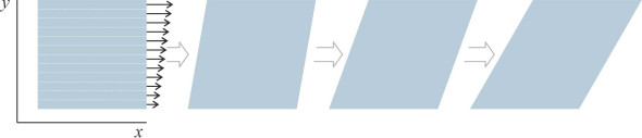
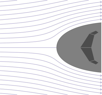
Liquids are hard to squeeze. Fill a container with water and press down on the surface as hard as you can - it won’t shrink, at least not enough for you to notice (figure 1). On the other hand, it won’t keep its shape. If you apply a shear force - which is not the same thing as squeezing - the water particles will slide over one another and you’ll feel very little resistance at all (figure 2). They are not completely frictionless: a viscous shear stress will occur between neighbouring layers if they are forced to move at different speeds. This is what happens when you skim a stone across a pond: the stone will bounce on the surface, and at each bounce, it drags some of the water particles along with it. These in turn drag some of the water particles in the layer below, and the relative motion sets up a frictional shear stress between the water and the stone. As a result the water speeds up while the stone slows down, the hops becoming progressively smaller until the stone loses all its kinetic energy in overcoming friction and sinks to the bottom. This kind of shear resistance is common to all fluids including gases like air. Any object moving through a viscous fluid will experience frictional ‘drag’ and, quite often, a transverse force as well, as shown in figure 3. To explain these forces, we’ll need to modify the flow theory that we’ve been working with until now.
Figure 1
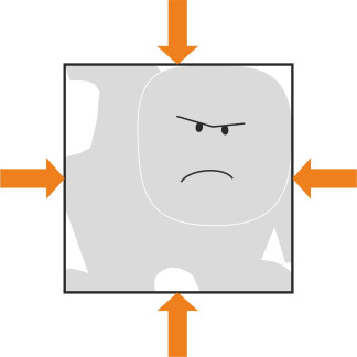
Figure 2
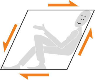
Figure 3
The viscous flow field
The first question is, how much shear stress can a fluid exert, and under what circumstances? We need a formula that links the shear stress in some way to the fluid motion. The first person to produce such a formula was Isaac Newton: his model is still used today, and a fluid that obeys the model is called a Newtonian fluid. The key is the rate at which the fluid is made to distort, in other words, the ‘velocity gradient’.
Figure 4
Shear stress
In figure 4 we see a chunk of fluid in which all the particles are moving in straight lines from left to right parallel to the \(x\)-axis. The layer at the bottom is moving at speed \(u\). The layer immediately above is moving slightly faster, and the one above that faster still. In fact there is a gradual increase in velocity with distance \(y\), measured at right-angles to the direction of flow, and the rate of increase is termed the velocity gradient. For a Newtonian fluid, we imagine the shear stress \(\tau\) anywhere in the fluid as being equal to the velocity gradient times a fixed constant. The constant is known as the ‘dynamic viscosity’ (or just ‘viscosity’ for short). It has units of [force] \(\times\) [time] / [area] (typically N s m\(^{-2}\)) and is denoted by \(\mu\):
(1)
\[\begin{equation} \tau \quad = \quad \mu \frac{du}{dy} \end{equation}\]In figure 4, the velocity profile (the line joining the tips of the arrows) happens to be a straight line with a constant slope so the shear stress between each layer and its neighbours has the same value from top to bottom across the flow field.
You might wonder where the shear stress comes from. It’s not immediately obvious how the layers can resist sliding over one another – they’re not like sheets of paper with rough surfaces that might dig into each other and interlock. The explanation lies in the behaviour of fluid particles at the molecular level. If the fluid happens to be a gas, the molecules are not all moving in the same direction – they dart about and collide with molecules in other regions nearby. In this way, particles from a slowly-moving layer (let’s call it ‘layer A’) will gain momentum from those in a faster-moving layer B alongside, causing the layer B to slow down a little. Conversely, particles from the layer B will cross into layer A and speed it up it a little. The effect is the same as if the layers were exerting a shear force on each other that tends to bring their velocities more closely into line. The mechanism is slightly different if the fluid happens to be a liquid: the molecules bunch together so they are less inclined to cross the streamlines between neighbouring layers. But as explained in Section F2019 they carry electrostatic charges that attract other molecules nearby and as a result, resist distortion in shear.
The Navier-Stokes equations
It is hard to predict the behaviour of a viscous fluid because the friction between neighbouring layers complicates the equations of motion. You may recall how we worked out the equations of motion for a non-viscous fluid, the Euler equations, in Section F1918. Let’s see if we can apply the same procedure to a viscous fluid. Essentially, we picture the flow field as a three-dimensional array of box-shaped elements, each containing a fluid particle on its journey through the flow field. There are countless particles, all undergoing forces and accelerations that are slightly different but mutually self-adjusting. For a typical particle we write down an expression for each of the forces acting on it, sum all the forces, and finally apply Newton’s Second Law of Motion to get a set of equations describing how the applied force, the mass of the particle and its acceleration are related. These constitute the basic equations of motion for the flow field, and if we can solve them, they will give us a picture of the fluid motion around a body moving through it. For a viscous fluid, the equations look similar to the ones set out in Section F1918, except that they include some additional terms that describe the shear forces acting on each face of the fluid element.
These are the Navier-Stokes equations we referred to in the opening Section of this series on fluid mechanics. If you’re interested, you’ll find them in the Appendix to this Section. The precise formulation varies with the assumed properties of the fluid; here, we assume an incompressible fluid in steady, laminar flow. Unlike the Euler equations, which we were able to solve at least for simple body shapes such as a circular cylinder, the Navier-Stokes equations have very few known solutions and therefore can’t be used to predict the pattern of flow around a moving vehicle. The equations, particularly as they relate to turbulent flow, have been a subject of intensive research for many years. In the year 2000, the question of how to solve them was recognised by the Clay Mathematics Institute in the USA as among the seven most difficult mathematical problems of our time; the Institute has offered a prize of $1 million for a proof that solutions exist and that they are unique [6].
Figure 5
It was the difficulty of solving these equations that in 1904 led a young German scientist called Ludwig Prandtl to find an ingenious way round the problem. In many situations, the flow field can be separated into two distinct parts. See, for example, what happens at the front of a moving vehicle. At first glance, the pattern of motion is not very different from the ‘potential flow’ we observed in Section F1919 for a frictionless fluid. In the regions that are remote from the boundary surface, the fluid particles are unaffected by skin friction, and they deflect around the body following smoothly curved streamlines in much the same way (figure 5). What’s different is the flow next to the body surface.
The boundary layer
Prandtl realised that the fluid molecules at the interface would be electrically attracted to the body surface and (as experiments have since confirmed) they would come to a halt. Since the fluid is viscous, there must be a slow-moving layer next to the vehicle skin, because the stationary particles exert a shear force on the adjacent fluid layer. The adjacent layer slows down a little, and this in turn slows down other particles further away. Together, the affected fluid particles constitute a boundary layer, outside which the motion is largely unaffected. The layer itself may be very thin, but it exerts a frictional force that opposes the vehicle’s motion.
Figure 6
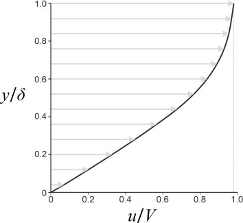
When a fluid moves in contact with a real object such as an aircraft wing, its velocity profile is not actually a straight line. Figure 6 shows how it varies close to the surface of a flat plate aligned parallel to the flow. You’ll notice that the curve passes through the origin; here, the velocity \(u\) must be zero in order to satisfy the ‘no-slip’ assumption mentioned earlier. Its value rises with increasing distance \(y\) from the wall, gradually approaching the velocity \(V\) of the undisturbed stream. It never quite gets there, so by convention we define the edge of the boundary layer as the point where \(u\) reaches a value equal to \(99\%\) of the undisturbed velocity. The thickness of the boundary layer measured in this way is denoted by \(\delta_{99}\) or just \(\delta\) for short. What determines the shear stress on the plate is the velocity gradient \(du / dy\) at the boundary wall where \(y = 0\), together with the dynamic viscosity \(\mu\). According to equation 1, the shear stress equals the product of the two. The shear stress acting on each square millimetre, when summed over the whole area of the plate, leads to a resistance force, one that is often called skin friction to distinguish it from other forms of resistance.
Since the fluid is applying a shear force to the plate, the plate must exert an equal and opposite shear force on the fluid whose effect is to slow down particles in the boundary layer. Imagine that we inject some coloured dye into a blob of particles within the boundary layer and track their progress along the body surface. They will gradually slow down as they move downstream, and through viscous friction, retard more particles alongside. The result is that, starting from zero at the leading edge of the plate, the thickness of the boundary layer increases gradually towards the rear, while the average velocity falls.
Modelling viscous flow
The division between the ‘remote’ flow field and the boundary layer is, of course, artificial, because the two merge imperceptibly into one. Nevertheless, the boundary layer is a useful idea, especially for streamlined bodies operating at high Reynolds numbers. In principle, one can start by modelling the flow pattern in the wider flow field using potential flow theory - as if the boundary layer does not exist. The next question is how to handle the boundary layer itself. Prandtl’s insight was to realise that a thin boundary layer can be represented as a two-dimensional slice. Under these conditions, a small degree of curvature can be neglected, as if the flow were taking place along the surface of a flat plate [24]. One can then assume that the pressure at any location is uniform over the whole depth of the boundary layer, which greatly simplifies the Navier-Stokes equations, enabling the investigator to deduce the shear forces acting on the body surface. To summarise, all you have to do is to analyse the two regions separately, starting with the inviscid flow model. The inviscid model will yield estimates of the fluid pressure and velocity at each point along the boundary surface, and these estimates can be used as input to the boundary layer model, a process called ‘patching’.
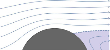
The approach works well for streamlined shapes such as an aircraft wing, this being the particular problem that Prandtl and his colleagues were working on. But it’s not appropriate for a blunt body such as an automobile, because the fluid viscosity leads to another phenomenon that completely transforms the flow field. For reasons we’ll mention later, at some point towards the tail (or at any sharp corner) the boundary layer will detach itself from the body surface and form a turbulent wake. Interestingly, separation will occur even in a fluid with vanishingly small viscosity, so it can’t be ignored.
Turbulence
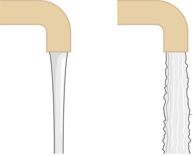
Flow that takes place smoothly and steadily in the manner described is called ‘laminar flow’, and it generates a modest level of resistance. But laminar flow is not very stable, and it breaks down when the rate of shear distortion reaches a certain intensity. Since the fluid particles don’t stick firmly together, the motion will become disorderly, with random fluctuations in speed and direction superimposed on the original flow pattern. You will have seen this happen many times. When you turn on a water tap, assuming you open it gradually, the flow will appear smooth and laminar (figure 7). As you open the tap further, at some point it will change into an agitated stream.
Figure 7
Reynolds’ number
The breakdown of laminar flow has a dramatic effect on the fluid’s behaviour so it’s useful to know where and under what circumstances it is likely to take place. It’s a problem that has excited the curiosity of scientists and engineers for over a hundred years. The first step was taken by a Victorian eccentric who combined an interest in natural philosophy with a gift for tackling engineering problems at a practical level. Fascinated by eddies, vortices and turbulence, Osborne Reynolds (1862 - 1912) worked on the problem during the 1880s and observed a common pattern in the behaviour of different fluids of different viscosity flowing along pipes of different size. The critical velocity was proportional to the pipe diameter and inversely proportional to the viscosity of the fluid [10]. His findings can neatly be summarised in terms of the dimensionless quantity known as the Reynolds Number:
(2)
\[\begin{equation} \operatorname{Re} \quad = \quad \frac{\rho VL}{\mu } \quad \text{or} \quad \frac{VL}{\nu } \end{equation}\]where \(\rho\) is the fluid density, \(\mu\) the (dynamic) viscosity, \(\nu\) the kinematic viscosity, \(V\) the fluid velocity averaged over the pipe cross-section, and \(L\) a typical dimension, in this case the pipe diameter. We’ll be learning more about the Reynolds number and why it takes this particular form later in Section F1817.
The Reynolds number is the most widely used parameter in fluid mechanics today. Its value tells you a lot about the nature of the flow and in particular whether the boundary layer is likely to be laminar or turbulent, and it’s this aspect that we’ll focus on here. For pipe flow, Reynolds discovered that the transition took place at a critical value \(\operatorname{Re}_{crit}\) of a little over 2 000. In other situations, \(\operatorname{Re}_{crit}\) has a different value. For a moving body immersed in a fluid, it is much higher, partly because the parameters \(V\) and \(L\) must be defined in a different way, with \(V\) as the velocity of the undisturbed stream, and with \(L\) usually taken as the length of the body measured parallel to the flow. Even then it is not a fixed number but varies according to the shape of the moving body, the roughness of its surface, and whether the wider flow field is itself free of turbulence. For the moment we’ll assume a value of around \(5 \times 10^{5}\) [21] [33].
Based on this assumption, we can predict the state of the boundary layer around any moving body by estimating the value of the Reynolds number and comparing it with the critical value \(5 \times 10^5\). For insects in flight, both \(V\) and \(L\) are small so the Reynolds number is small too: around 7 000 for a gliding butterfly for example [31], down to less than 20 for a tiny parasitic wasp [8]. These values are well below the critical value, so the flow is smooth and laminar. At the opposite end of the spectrum, for moving vehicles the situation is very different. Take, for example, a saloon car. It is larger and travels much faster than a butterfly, and at a cruising speed of 30 m/s its Reynolds number is of the order of \(1.0 \times 10^7\), which is well above the critical value for turbulent flow. As shown in table 1, the Re values for other types of vehicle are higher still, of the order \(10^{8}\) or \(10^{9}\). In the world of mechanical transportation, turbulent flow is the norm.
| Vehicle | Fluid | Kinematic viscosity (\(m^{2}s^{-1}\)) | Length (\(m\)) | Speed (\(m/s\)) | Reynolds number |
| Saloon car | Air | \(14.6 \times 10^{-6}\) | 5.0 | 30 | \(1.1 \times 10^{7}\) |
| Intercity railway train | Air | \(14.6 \times 10^{-6}\) | 500.0 | 60 | \(2.1 \times 10^{9}\) |
| Container ship | Water | \(1.0504 \times 10^{-6}\) | 300.0 | 6 | \(1.7 \times 10^{9}\) |
| Jet airliner (fuselage) | Air | \(14.6 \times 10^{-6}\) | 70.0 | 250 | \(1.2 \times 10^{9}\) |
| Jet airliner (wing) | Air | \(14.6 \times 10^{-6}\) | 8.8 | 250 | \(1.5 \times 10^{8}\) |
Figure 8
The break-down
None of the foregoing, however, explains why the flow breaks down. The formula for the critical Reynolds number (equation 2) hints that it might be something to do with speed: by definition, anything that moves fast has kinetic energy that (metaphorically speaking) can spill over and cause a disturbance. However, in the case of a moving fluid the explanation is more specific. The criterion cannot be speed alone: at breakfast, your coffee cup rests on a table that is being carried on a planet circling around the sun at a speed of 30 km/s, many times faster than the speed of sound. Yet the coffee inside is perfectly stable. What matters is not the speed alone, but the speed coupled with shearstrain, the graduation in speed between neighbouring layers of fluid that we pictured earlier in figure 4. It occurs not only within a boundary layer, but as we’ll see later, in other situations that don’t involve a solid surface.
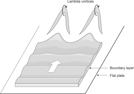
The simplest form of boundary layer is one in which the fluid moves in laminar fashion (at least initially) along a smooth, flat plate aligned parallel with the oncoming flow. What might trigger turbulence? During the nineteenth century, the eminent physicists Reynolds and Rayleigh were among the first to investigate the phenomenon, but they couldn’t predict whereabouts on the body surface the transformation would take place. Only in 1930 did two of Prandtl’s former students, Walter Tollmein and Hermann Schlichting, succeed in developing a theoretical procedure for doing so. Since then, many years of research have revealed an intriguing chain of events that occur during the process at a microscopic level. There are four main stages, of which the first two are shown diagrammatically in figure 8:
- During the first stage, regular perturbations occur in the form of two-dimensional transverse waves called Tollmein-Schlichting waves [18] [29]. They extend along 80\(\%\) of the transition region.
- The waves transmute into tiny three-dimensional vortices known as ‘\(\Lambda\) -structures’.
- The vortices soon decay into patches or ‘spots’ of turbulent flow.
- The ‘spots’ merge into a fully developed turbulent boundary layer.
A more detailed description including photos of the vortex structure can be found in [12] [30] [34]. For some time now, investigators have been trying to account for the breakdown through computer simulation and mathematical models. One particular model draws on a body of theory whose origins lie outside the realm of fluid mechanics. It has evolved over the last few decades to handle a range of physical processes that evolve over time: in other words ‘dynamical systems’. It deals with stability of the system as a whole rather than the underlying physics, in response to gradual changes over distance or time in one of the underlying parameters that control its behaviour. When the parameter reaches a critical value, the equations of motion have more than one solution and the system is forced to ‘choose’ one of the available states or oscillate between them, a process known as bifurcation. Successive bifurcations can lead to a chaotic state such as turbulence (here the term ‘chaos’ has a precise mathematical meaning).
This is essentially what happens to a fluid when the Reynolds number reaches the critical value that marks the transition to turbulent flow. Dynamical systems theory can help one make sense of other fluid phenomena such as the oscillating vortex street generated by a circular cylinder arranged at right-angles to the fluid flow, a phenomenon that we’ll touch on briefly later. Stability theory is a challenging subject in its own right, and we won’t pursue it any further here, but for more information about its application to fluid flow, you want might to consult a specialist source, for example [13].
When a boundary layer becomes turbulent, the frictional drag increases, so it is important to know whether turbulence is likely to occur in the flow around a vehicle. If so, a key parameter is the distance \(x_{crit}\) of the point at which the transition takes place measured from the front of the vehicle. To estimate this distance, we’ll assume that the vehicle has a slender, streamlined profile so the boundary layer behaves like the boundary layer on a flat plate. Experiments have shown that for a flat plate with a polished surface and a sharp leading edge, the critical Reynolds number can be as high as \(3 \times 10^{6}\). But vehicles are not actually as smooth as you might think, even the surface of an aircraft wing, which is punctuated by rivet heads together with small insects whose carcasses become glued to the surface on impact. Such irregularities protrude into the boundary layer and disturb the flow. In addition, the approaching fluid itself may contain a degree of turbulence arising from some other source. Under these conditions, the critical Reynolds number may fall to \(2 \times 10^{5}\) [21], although for practical purposes it is common for engineers to assume a value around \(5 \times 10^{5}\) [21] [33].
We can get a rough estimate of \(x_{crit}\) from equation 2. Given a flat plate immersed in a flow whose free stream velocity is \(V\), the equation tells us how the Reynolds number varies with the length \(L\) of the plate. If we fix the value of Re at its critical value \(5 \times 10^{5}\), we can turn the equation around and it will tell us the length of plate at which the flow just becomes turbulent, which is just the value \(x_{crit}\) that we are looking for:
(3)
\[\begin{equation} x_{\text{crit}} \quad = \quad \left( 5 \times {10}^{5} \right) \times \frac{\nu }{V} \end{equation}\]where \(V\) is the free stream velocity relative to the plate and \(\nu\) the kinematic viscosity. For the saloon car travelling at 30 m/s as detailed in table 1, this distance works out at \(0.0000146 \times 500 000 / 30 = 0.24\) m, suggesting that for a saloon car at cruising speed, transition takes place only a few centimetres from the nose. For other vehicles detailed in the Table, the corresponding distance is shorter still. Hence for moving vehicles the boundary layer is turbulent along most of the body surface.
Turbulent flow
We don’t yet have a complete description of turbulent flow. It can be pictured as a three-dimensional jumble of eddies and vortices, all short-lived, with pattern of movement that is repeated like a fractal on different physical scales. Energy is dissipated by the smallest eddies at the bottom of the scale. The diameter of the largest eddies is limited to about half the thickness of the boundary layer. In the case of an aircraft wing, the boundary layer is only a few millimetres thick, so the eddies are small. In the case of a 300 m-long container ship, the boundary layer is typically around a metre thick at the stern, so the eddies are much larger. In fact it’s easier to characterise eddies in terms of their time duration rather than their physical dimensions: in marine hydrodynamics, the velocity variations occur at frequencies 1 Hz and above, with amplitudes around \(10\%\) of mean velocity [15] [19]. On a larger scale are the variations that occur within the earth’s atmosphere. The wind that blows along the street outside your house represents the boundary layer that stretches across the earth’s surface. Because it’s disturbed by hills, trees and buildings, the motion is turbulent, and measurements with instrumented kites have shown that the flow breaks up into elongated structures - ‘turbulence sausages’ - each of which spins around its major axis. The largest eddies observed on this scale have periods of the order of one minute [7].
In a turbulent boundary layer, the particles no longer travel at a constant speed, nor in a fixed direction parallel to the boundary surface. It is conventional to represent the fluid motion with streamlines, but these are ‘average’ streamlines that individual particles cross and re-cross on their journey downstream. Moreover, random motion in the \(y\)-direction implies there is mixing between layers. We’ve already touched on the mixing that occurs when the molecules in a gaseous fluid cross between neighbouring layers, and how this mixing is responsible for the fluid viscosity in laminar flow. But in turbulent flow, the mixing occurs on a much larger scale and it occurs in liquids too: the momentum transfer involves not just individual molecules but whole lumps of fluid. Hence the layers interact as if the viscosity has greatly increased, so that turbulence raises the effective viscosity by several orders of magnitude [1].
Figure 9
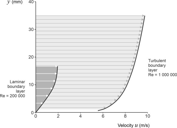
We can draw a velocity profile for a turbulent boundary layer like the one shown earlier in figure 6 for the laminar case. We do this on the understanding that the ‘velocity’ now represents the average component of velocity \(u\) in the \(x\)-direction. Figure 9 shows the profile for a turbulent boundary layer at a point 1.5 m from the leading edge of a flat plate aligned parallel to the air flow with the Reynolds number fixed at \(10^6\). The smaller curve on the left hand side is the velocity profile for laminar flow at the same location, with the Reynolds number reduced to \(2 \times 10^5\) (this is the same profile as the one previously shown in figure 6, but scaled to reflect the above flow parameters). For the turbulent flow you can see that the boundary layer is thicker because it entrains more fluid, and the velocity gradient at the wall is more severe. Hence the shear stress between the fluid and the boundary surface is greater and the drag must increase. Less obvious is the existence of a thin sub-layer next to the wall where the flow remains laminar provided the plate is smooth. It’s not really a distinct layer, but a reflection of the fact that here, there can be no velocity fluctuations in the \(y\)-direction because the boundary itself gets in the way. Since the fluid particles can only move parallel to the surface, the momentum transfer diminishes to zero and there is no turbulence. The velocity profile for this layer is not shown in the Figure.
Skin friction
During the nineteenth century, physicists and engineers could predict the motion of a fluid only on the assumption that it was friction-free. Any viscous interaction between the fluid layers must radically alter the flow pattern, and no-one knew how to solve the Navier-Stokes equations that governed viscous behaviour. But a way round the impasse appeared in 1904, when Ludwig Prandtl (1875-1953), then a young Professor of Mechanics at the Technische Hochschule in Hannover, realised that for a streamlined shape such as an aircraft wing, the effects of viscosity were confined to a thin layer close to the wing surface, in other words, a boundary layer. He set out his ideas in a paper that is now world-famous but for almost 20 years was ignored outside Germany [14]. The boundary layer concept enabled engineers to estimate the frictional drag of an aircraft wing; Prandtl went on to make further discoveries, and while he was doing so, trained a cohort of research students who pioneered the science of aerodynamics as we understand it today.
Friction in a laminar boundary layer
Prandtl’s first task was to put together a model for the boundary layer over a flat plate assuming laminar flow. He was able to simplify the Navier-Stokes equations by treating the boundary layer as a two-dimensional phenomenon, sufficiently thin to make the pressure variations across the boundary layer and motions perpendicular to the boundary surface negligible. A solution was now in sight, and at this point Prandtl shared the problem with one of his research students, Paul Richard Heinrich Blasius (1883 – 1970). Blasius reasoned that the velocity profile should have the same geometric form at all locations along the plate, appropriately scaled in the \(x\) and \(y\) directions, and applied a coordinate transformation that reduced the problem to single, ordinary differential equation which could be solved numerically to yield the velocity profile. You can find his table of results reproduced in [33], and these are the results your author used to plot the velocity profile shown earlier in figure 6.
By evaluating the velocity gradient at the wall, one can derive an expression for the shear stress \(\tau_x\) acting on the boundary surface at a distance \(x\) from the leading edge of the plate [28]:
(4)
\[\begin{equation} \tau_w \quad = \quad 0.332 \rho V^2 \operatorname{Re}_x^{-\frac{1}{2}} \end{equation}\]The Reynolds number here is interpreted as \(Vx/\nu\), so equation 4 can be written in the form
(5)
\[\begin{equation} \tau_w \quad = \quad 0.332\rho V^{\frac{3}{2}} \nu^{\frac{1}{2}} x^{-\frac{1}{2}} \end{equation}\]As you’d expect, the shear stress increases with the speed of vehicle. On the other hand, at any given speed it decreases along the plate with the distance \(x\) from leading edge; this is because the velocity gradient at the wall isn’t constant: it declines steadily as the boundary layer thickens towards the rear. By integrating over the area of the plate, assuming it has width \(b\) and length \(l\), we deduce a total drag force given by
(6)
\[\begin{equation} D_{friction} \quad = \quad 0.664 \rho V^{\frac{3}{2}} \nu^{\frac{1}{2}} b l^{\frac{1}{2}} \end{equation}\]and an overall friction drag coefficient (we’ll explain what a drag coefficient is later, in Section F1817):
(7)
\[\begin{equation} C_{D,friction} \quad = \quad 1.328 \operatorname{Re}_l^{-\frac{1}{2}} \end{equation}\]where \(\operatorname{Re}_l\) is the Reynolds number for a flat plate of length \(l\) [33]. One can also deduce from Blasius’ results an expression for the boundary layer thickness \(\delta\):
(8)
\[\begin{equation} \delta \quad = \quad 5.0 x \operatorname{Re}_{x}^{-\frac{1}{2}} \end{equation}\]which can be written in the form
(9)
\[\begin{equation} \delta \quad = \quad 5.0 \nu^{\frac{1}{2}} V^{-\frac{1}{2}} x^{\frac{1}{2}} \end{equation}\]You can see from the right-hand side that the boundary layer thickness is not uniform along the length of the plate. Provided the Reynolds number is not too small, the thickness is zero at the leading edge and grows steadily with distance downstream as shown in figure 10 (the vertical scale has been exaggerated). Notice also the factor \(V^{-\frac{1}{2}}\): the faster the flow, the thinner the boundary layer as a whole. At first glance, this doesn’t make sense. You would expect that the faster a body moves, the greater the impact it must have on the surrounding fluid – surely the shear stresses propagate further afield? It makes even less sense if you turn the statement around: it implies that when a body slows down, the boundary layer deepens. But in fact this is what happens.
Figure 10
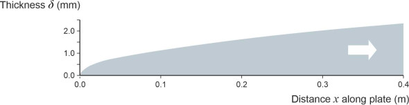
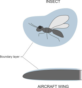
Shortly, we’ll outline a similar paradox in the context of a turbulent boundary layer, and try to explain what is going on, but for the moment, note that it’s consistent with our earlier observation that the boundary layer around an insect – for example a gnat - extends for an appreciable distance into the surrounding flow field. To give you an idea of what that means for the gnat, assume it has a wing chord of 1 millimetre and flies at 0.25 m/s in air whose kinematic viscosity is 0.00001461 m2 s\(^{-1}\), and substitute these values in equation 9. It predicts a boundary layer thickness of \(5.0 \times \left( 1.46 \times 10^{-5} \times 0.001 / 0.25 \right)^{\frac{1}{2}}\), which works out at a little over 1 mm, much thicker than the wing itself. Indeed, as shown in figure 11, the gnat is carrying around an air bubble much larger than its own body, and must feel like it’s swimming through water. On the other hand, the flow is laminar in spite of the insect’s body surface, which follows a series of bumps and indentations quite unlike the smooth contours of a bird or an aircraft. Effectively, the boundary layer acts as an aerodynamic outer shell. Whereas an aircraft has to be streamlined, bees and wasps don’t.
Figure 11
Friction in a turbulent boundary layer
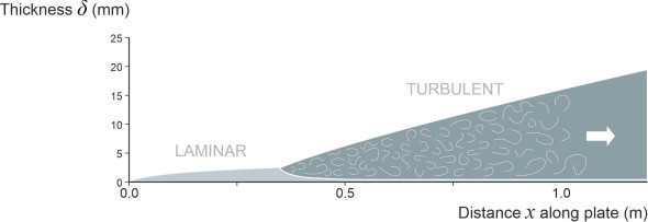
Assuming that the flow field is smooth and steady upstream, when fluid particles encounter a moving body they form a boundary layer that is laminar at the leading edge or nose. If the Reynolds number is small it remains laminar throughout its whole length, but even if the Reynolds number is large, it doesn’t become turbulent straight away. To see why, let’s carry out a thought experiment in which fluid is moving over a flat plate as previously shown in figure 10. The plate measures 1.5 m long in the direction of flow. The free stream velocity \(V\) starts at a very low value so the flow is laminar throughout. Now raise \(V\) by a small amount. As a result, the Reynolds number will increase too. If we continue to raise the velocity in small increments, eventually a change will occur in the profile of the boundary layer at the downstream end of the plate surface. The change marks the point of transition at at a distance \(x_{crit}\) from the nose where the flow becomes turbulent. If the velocity continues to rise, equation 3 shows that \(x_{crit}\) will fall and hence the transition point will move forward with each increment until it almost reaches the nose. At the end of our thought experiment the flow will be laminar at the nose but turbulent over the greater surface area of the plate: hence a turbulent boundary layer is always a composite of two distinct parts, although at high Re values, the first part – the laminar section – will be very short. Now let’s go back and examine the structure of the flow field at some intermediate stage. The cross-section is shown diagrammatically in figure 12 for the case where the transition point lies about a quarter of the way along the plate. Apart from an abrupt increase at that point, the thickness \(\delta\) of the boundary layer increases steadily in the downstream direction.
Figure 12
With this picture in mind, we can now see how the fluid particles interact with the boundary surface. Ahead of the transition point, the flow pattern is laminar and since it’s not affected by what happens downstream, the values of the shear stress and boundary layer thickness will be as predicted by equations equation 5 and equation 9 above. Hence we can focus on the rear section of the plate where the boundary layer is turbulent. As described earlier, when the flow becomes turbulent, a great deal more mixing occurs among the fluid layers. Effectively, the viscosity increases, and with it, the shear stress between neighbouring fluid layers. The ‘extra’ shear stress is often described as the Reynolds stress after Osborne Reynolds, who believed that the effects of turbulent mixing could be represented as an extra stress term in the Navier-Stokes equations. Unfortunately, Reynolds’ idea doesn’t work in the context of a boundary layer (in Reynolds’ day, no-one knew that boundary layers existed). So we can no longer use equation 1, which predicts the shear stress acting on a body given the velocity gradient at the surface. However, there is an alternative method that by-passes the problem altogether. It involves three main steps. First, you determine by experiment an empirical relationship between the shear stress and the boundary layer thickness \(\delta\). Within this relationship, the boundary layer thickness appears as an unknown. Second, you assume a velocity profile and work out the implied rate of loss of momentum per unit length of boundary layer in terms of \(\delta\). Finally, you equate the shear stress with the rate of loss of momentum to get an integral equation that can be solved to yield an expression for \(\delta\) in terms of \(V\) and \(x\). Explicit formulae for the shear stress and drag coefficient then follow.
The procedure is based on a mathematical technique originally conceived by von Karman as a tool for analysing laminar flow. Known as the momentum integral method, it exploits the fact that the results aren’t very sensitive to the shape of the velocity profile, so one can substitute a polynomial in place of Blasius’ table of numbers. The same method can be applied to a turbulent boundary layer as well. For turbulent flow, a commonly used velocity profile is the ‘one-seventh power law’, which was originally derived from experiments with pipe flow:
(10)
\[\begin{equation} \frac{u}{V} \quad = \quad \left( \frac{y}{\delta } \right)^\frac{1}{7} \end{equation}\]On this basis, one can use the momentum integral equation to derive formulae for the boundary layer thickness, shear stress, and drag for a turbulent boundary layer as follows. We’ll quote the ones set out in [22]; similar results with small differences in the numerical coefficients appear in other textbooks. The empirical shear stress is given by
(11)
\[\begin{equation} \tau_w \quad = \quad 0.0288 \rho V^{2}{\operatorname{Re}}_{x}^{-\frac{1}{5}} \end{equation}\]alternatively
(12)
\[\begin{equation} \tau_w \quad = \quad 0.0288 \rho V^{\frac{9}{5}} \nu^{\frac{1}{5}} x^{-\frac{1}{5}} \end{equation}\]As before, the shear stress declines gradually along the length of the plate. The total friction drag acting on one side of a plate of area \(A\), length \(l\) and width \(b\) is given by [22]:
(13)
\[\begin{equation} D_{friction} \quad = \quad 0.0360 \rho V^2 A {\operatorname{Re}_l}^{-\frac{1}{5}} \end{equation}\]Alternatively:
(14)
\[\begin{equation} D_{friction} \quad = \quad 0.0360 \rho V^{\frac{9}{5}} \nu^{\frac{1}{5}} b l^{\frac{4}{5}} \end{equation}\]while the friction drag coefficient is given by
(15)
\[\begin{equation} C_{D, friction} \quad = \quad 0.072 {\operatorname{Re}_l}^{-\frac{1}{5}} \end{equation}\]The boundary layer thickness is given by
(16)
\[\begin{equation} \delta \quad = \quad 0.370 x {\operatorname{Re}_{x}}^{-\frac{1}{5}} \end{equation}\]or alternatively
(17)
\[\begin{equation} \delta \quad = \quad 0.370 \nu^{\frac{1}{5}} V^{-\frac{1}{5}} x^{\frac{4}{5}} \end{equation}\]which by comparison with equation 9 shows that the thickness grows more quickly with distance downstream than in the laminar case. But it’s still small compared, for example, with the thickness of an aircraft wing. In the case of a medium-sized passenger jet whose wing cross-section measures around 5 m from the leading edge to the trailing edge, at a cruising speed of 250 m/s the boundary layer reaches a maximum depth at the trailing edge of only around 50 mm. This is small compared with the thickness of the wing itself, typically 600 mm for a wing of this size.
Although they are only approximations, equations equation 11 - equation 17 help one to identify the variables that affect the boundary layer, and by how much. Using them, one can easily gauge what would happen if the length of a moving vehicle, for example, were increased by say 20 percent, or if the speed were to double. But being empirical models, they don’t really explain what is happening inside the boundary layer itself. Prandtl and his colleagues eventually worked out separate models for the outer region and the laminar sub-layer that were more firmly rooted in fluid flow theory, and fitted a logarithmic curve that joined them smoothly together in the middle region. Not surprisingly perhaps, the mathematics is challenging, and you can find out more in [32] [27].
There is however a particular feature of equation 17 that looks odd: the factor \(V^{-1/5}\). As in the laminar case, it seems that when a vehicle speeds up, the thickness of the boundary layer must fall. The relationship is so weak in this case that it won’t fall much, but nevertheless the effect is counterintuitive. The explanation lies in the fact that there are several distinct forces at work in any flow field, of which the most important are usually (a) viscous forces and (b) inertial forces. The viscous forces derive from the ‘stickiness’ of the fluid, and they discourage adjacent layers from sliding over one another. The inertial forces, however, are related to momentum. You can see fluid momentum in action when you turn on a garden hose. The water gushing from the nozzle can knock over a flower pot. When the water particles collide with the pot they lose momentum, and it’s the rate of change of momentum that determines the force acting on the flowerpot surface.
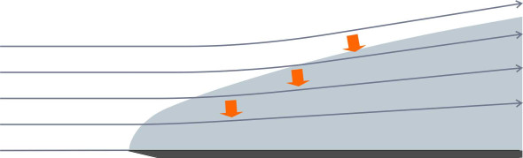
In the Appendix to this Section, we’ll see how the forces are linked to individual terms in the Navier-Stokes equations, and we’ll be examining their origins in more detail later in Section F1817, but for now let’s return to the flat plate. If the velocity \(V\) of the fluid stream changes, the balance between the viscous force and the inertial force changes too. It turns out that the viscous force is proportional to \(V\), while the inertial force is proportional to \(V^2\). So as \(V\) increases, the viscous component increases less quickly than the inertial component, and therefore at high Reynolds numbers, the inertial component dominates. In this particular set-up, the inertial forces don’t act directly on the plate because it is aligned parallel to the oncoming flow: when viewed from the front, it barely obstructs the flow field and there is nothing with which the fluid particles can collide. However, the boundary layer itself is a kind of obstruction. Because the fluid it contains is moving more slowly than the fluid outside, the boundary layer behaves as an extension of the plate and effectively turns it into a three-dimensional ‘body’. It has a frontal ‘area’ that can be quantified in terms of a mathematical construct called the displacement thickness [20]. The inertial force acts on the nose of this virtual ‘body’ in almost the same way as it might act on the nose of an aircraft. You can see that when they enter the boundary layer, the streamlines diverge away from the plate surface as shown in figure 13 - they have to, because the fluid particles are slowing down. But at the same time, the inertia of the particles tends to carry them straight ahead, and the faster they are moving, the less the angle of deflection. In simple terms, the oncoming particles flatten the boundary layer, squeezing it more tightly against the wall.
Figure 13
The wake behind a moving body
Prandtl’s great idea was to divide the flow field around a moving vehicle into two distinct zones – a viscous boundary layer embedded within a potential flow – and analyse them separately. The technique works for any streamlined shape such as an aircraft wing because the boundary layer is thin, almost as if it were glued onto the wing surface. But it doesn’t work for a ‘bluff’ body with bulbous contours, particularly if it is squared off at the stern. Almost all passenger cars and railway trains come into this category. At some point along the body surface the boundary layer will break away, and from this point onwards, the nature of the flow field changes. The particles within the wake no longer converge smoothly behind the vehicle as they would in laminar flow, but rather, they form a wake. Inside the wake, the fluid motion may take on one of three distinct patterns: turbulent eddies, rotating ‘bubbles’, or a vortex street. Along the outer edges of the wake there is a steep velocity gradient across the ‘shear surface’ that separates it from the surrounding flow field. And elsewhere there may be helical vortices trailing from corners in the bodywork.
Figure 14
Separation
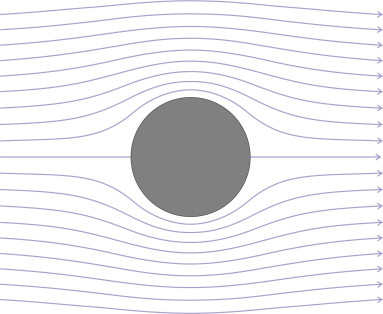
We’ll see in a moment that separation tends to occur wherever there is an abrupt angle in the vehicle bodywork or a sharp projection on the body surface. However, it also occurs on bodies with no sharp corners at all such as a football or a sports car. The reason can most readily be explained through an example, and the one we’ll use is a circular cylinder aligned at right-angles to a uniform flow field (figure 14). Let’s start off by imagining the flow is friction-free. Since the body is symmetrical fore-and-aft, the pattern of streamlines will be symmetrical too. Let’s see what happens to the fluid particles as they progress around the cylinder surface: specifically, we can track the different kinds of energy that the particles possess during their journey. In principle there are three kinds, pressure energy, kinetic energy, and potential energy, respectively represented by the three terms on the left-hand side of the Bernoulli equation:
(18)
\[\begin{equation} p + \frac{1}{2} \rho U^{2} + \rho gz \quad = \quad C \end{equation}\]in which \(U\) represents the fluid velocity locally along the streamline, and \(C\) is a constant having the same value throughout the flow field. The third term on the left reflects the gain or loss in pressure associated with a change in height. It is usually quite small so for present purposes we’ll ignore the third term and concentrate on the first two. Imagine a particle starting out from the upstream stagnation point, which is labelled S1 in figure 15. At that point, the fluid velocity \(U\) is zero and the pressure \(p\) is the ‘stagnation pressure’, the maximum possible value in this flow field, and numerically equal to \(C\).
Figure 15
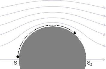
Suppose the particle moves clockwise over the top the cylinder. The pressure at the top of the cylinder is less than the stagnation pressure at S1 (a formula showing how the pressure varies around the cylinder surface appeared earlier in Section F1918, but you can see what is happening from the way the streamlines crowd together). Hence, propelled by the pressure gradient, the particle will speed up as it ascends, and as it does so, it will gain kinetic energy but lose pressure energy. At the summit, the pressure energy is at a minimum and the kinetic energy at a maximum – the flow is fastest here. As the particle continues down the rearward face, it will slow down again and the pressure will rise, until the particle comes to a halt at the rear stagnation point S2. Notice that the pattern of flow over the rear half of the cylinder is a mirror image of the flow pattern over the front half.
All well and good. But if we now replace the inviscid fluid with a viscous one, any particles making the journey between S1 and S2 will be affected by friction, and lose some energy en route. The energy will be dissipated as heat. So like a car running out of fuel, the particles will run out of kinetic energy before they reach their destination. Against a rising pressure gradient, the boundary layer will come to a halt and break away from the cylinder surface as shown in figure 16. Beyond this point the boundary layer reverses direction, and the dashed line indicates where the two streams meet. Let’s pause for a moment and think about what is happening. At first, the pressure gradient is ‘favourable’ – it pulls the fluid onwards, and draws the boundary layer firmly onto the cylinder surface. In this region, the flow pattern follows quite closely the streamlines predicted by inviscid flow theory. Later, on the downstream face the pressure begins to rise again and the gradient becomes ‘adverse’. This is the region where the boundary layer is liable to separate.
Figure 16
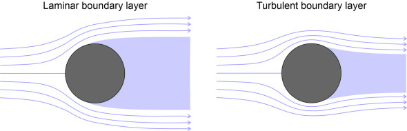
So far we have said nothing about whether the boundary layer is laminar or turbulent, and what effect this might have. In the laminar case, experimental studies of flow round a circular cylinder have shown that separation takes place earlier than you might expect, at a point slightly ahead of the top of the cylinder where the pressure gradient switches from favourable to adverse (figure 17). But for the sorts of vehicle we are interested in, the boundary layer is usually turbulent, and we would expect the separation to occur further aft. Indeed this is the case, and it happens because in turbulent flow, the fluid particles move randomly between layers and transfer kinetic energy from one to the other as they do so. The result is a continual boosting of the mean velocity in the x-direction of the layers closest to the boundary surface as they draw energy from the outer flow field. This replaces some of the energy lost to friction and delays the point where they come to a halt [25].
Figure 17
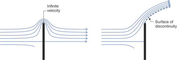
For bodies with a more complicated shape such as a moving vehicle, it is not easy to predict where the boundary layer will separate. One way to find out is to test its aerodynamic behaviour in a wind tunnel. Since turbulent flow is noisy, in a wind-tunnel experiment one can detect the point of separation with a stethoscope. Alternatively, the separation process can be simulated with CFD software. You can be sure about one thing, though. The boundary layer will detach itself wherever it meets a projection or a sharp corner on the body surface, such as a wing mirror. A wing mirror on an old-fashioned car resembles a flat plate. Aligned at right-angles to the oncoming airflow, it represents almost the least ‘aerodynamic’ shape one can imagine, and is an interesting case in its own right. Figure 18 shows the flow pattern over and under the plate around mid-section. Let’s see what happens at the top. If we regard the fluid as inviscid, we can use potential flow theory to predict the pattern of streamlines. It can be shown that they bunch close together where the flow curls around the edge, so the particles must be moving very quickly at this point. Indeed, if the plate has infinitesimally small thickness the velocity at the tip will be infinite. Hence we have a mathematical singularity that no real fluid can accommodate – one would expect it to separate at the top of the plate to produce a surface of discontinuity that extends outward into the flow field as shown on the right-hand side of figure 18, and another one, its mirror image, at the bottom. On either side of the discontinuity surface, the fluids are moving at different speeds. So we’ve removed the singularities, but at a price.
Figure 18
Shear layers
The idea of a surface of discontinuity puzzled scientists, who didn’t believe that an abrupt jump in velocity was possible: it didn’t conform to the laws of fluid motion as they were understood at the time. But around the middle of the nineteenth century, the eminent physicist Gustav Helmholtz found a way to represent two layers of fluid sliding over one another by means of an abstract mathematical device known as a vortex sheet. A vortex sheet is a row of line vortices of infinitesimally small diameter, packed side by side as shown in figure 19 [9]. Rotating very quickly like rollers under a conveyor belt, they allow a layer of fluid to slide over a neighbouring layer without violating Euler’s equations. Helmholtz showed that by adding the potential flow fields of an infinite number of vortices arranged in this way, the result was a discontinuous shear surface that Prandtl later demonstrated would curve downstream as shown in figure 18 [11].
Figure 19
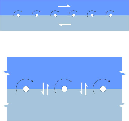
If all you need is an abstract model, the rollers seem like a good idea: they smooth out the interface so that mathematically speaking, the discontinuity is resolved. But it doesn’t explain the physics, for two reasons. First, a single row of point vortices evenly distributed along a shear surface is unstable [16]. Second, it doesn’t work mechanically. If you assemble a handful of metal rollers into a flat plane and pack them tightly together, they rub against each other as shown in the lower half of figure 19. In fact you have replaced a horizontal sliding interface with a lot of vertical ones!
An engineer would approach the problem differently. Why not make the rollers mesh like gear wheels without any shearing action at all? In principle, this could be achieved as shown in figure 20, with a fractal set containing an infinite number of rollers of ever-decreasing size. The orange rollers rotate clockwise while the blue ones rotate anticlockwise. At the top is a horizontal layer that moves from left to right at speed \(u\), say. At the bottom is a similar layer that moves at the same speed \(u\) but in the opposite direction. The two layers slide freely relative to one another because they don’t touch any blue rollers, only the orange ones. The arrangement of rollers is ad hoc but it seems to be repeatable down to an infinitesimally small scale, so they fill the entire space between the top and bottom layers, although only the larger rollers are shown in the diagram.
Figure 20
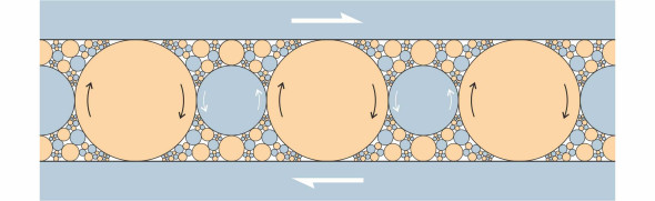
A set of rollers arranged like this has three distinguishing properties:
- the outer surface of each roller moves at the same speed \(u\)
- there is no sliding contact so the rollers generate zero friction
- it can be shown that the kinetic energy stored in each roller is proportional to its cross-sectional area, so that in a particular sense, the energy is distributed evenly across the breadth and length of the roller complex.
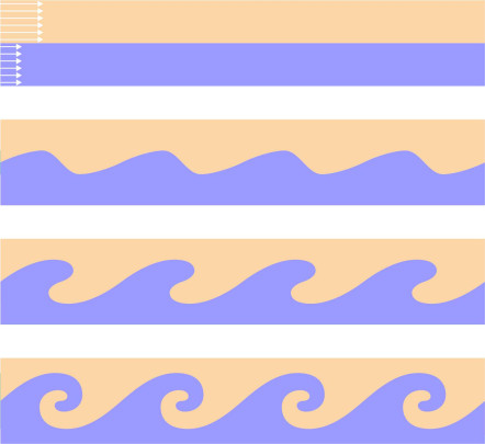
The fractal roller set is not a realistic model of fluid flow because fluid particles don’t readily organise themselves into a regular geometric pattern. At the interface between two layers, the velocity gradient de-stabilises the fluid particles so that the two fluid masses intermingle. Under ideal conditions, the process may begin with the formation of regular waves as shown in figure 21, but the waves progressively roll up and decay into eddies of different shapes and sizes whose progress is hard to define. A spectacular example of this phenomenon occurs high above the earth where jet streams pierce through the atmosphere at speeds approaching 150 km/h. The discontinuity between the edge of a jet stream and the surrounding air mass creates turbulence on a large physical scale. If you are flying in an aircraft and it strays into this zone, you will experience turbulent flow, as it were, from the inside: sometimes, an eddy will buffet the rudder and shake the fuselage from side to side. On a smaller scale are the shear layers created by an automobile. A turbulent shear layer will form wherever the boundary layer detaches itself from the body surface owing to the velocity gradient between the separated fluid and the body of ‘dead air’ immediately aft.
Figure 21
So the fractal roller model is just an analogy, which you may or may not find more convincing that the vortex sheet. However, we know that the mixing process in turbulent flow has a fractal element. The meteorologist Lewis Richardson once described atmospheric storms as ‘whirls’ of different size exchanging energy between them on a scale of descending size, with large eddies passing on energy to smaller ones, and then to smaller ones still – hence the famous quotation at the beginning of this Section. This idea that turbulent energy is passed down a kind of ‘ladder’ to smaller and smaller disturbances has intrigued scientists for some time, and a recent computer simulation experiment seems to support the idea [4].
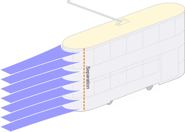
What happens in the wake
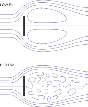
When a bluff body moves through a fluid at speed, the boundary layer may separate from the body surface, usually towards the rear. The place where the boundary layer separates marks the beginning of the wake (figure 22). The wake is a region where the fluid particles move less briskly than those outside, as if being dragged along behind. Exactly how they behave depends on the shape of the body and how fast it is moving, and to give you some idea of what can happen we’ll look at three examples, starting with the one that we looked at earlier: a flat plate aligned at right-angles to the flow.
Figure 22
The fluid in the region behind the plate is often referred to as ‘dead air’ or ‘dead water’; it moves sluggishly under the influence of the faster moving particles within the shear layers above and below. At low Reynolds numbers, the result is a pair of ‘separation bubbles’ that rotate inside the wake (figure 23). At higher Reynolds numbers, the separation bubbles break down into a confused, a turbulent wake. In both scenarios, the fluid pressure within the wake is significantly lower than that of the surrounding flow field. Hence the normal pressure acting on the downstream face of the plate no longer balances the pressure acting on the front, and together they generate a net drag force. It is called form drag, and is quite distinct from any shear force generated by boundary layer friction, although both are attributable to the fluid viscosity. Notice that in the case of the flat plate, the wake has a large cross-sectional area, so the form drag is considerable; in fact a flat plate aligned at right-angles to the fluid flow represents one of the least aerodynamically efficient body shapes one can imagine. It’s all form drag. Fluid moving up or down the front of the plate creates a shear stress, but it acts at right-angles to the direction of motion and doesn’t contribute to friction drag.
Figure 23
For the second example, we’ll return to the circular cylinder aligned with its axis at right-angles to the oncoming fluid stream. It is what aerodynamicists call a ‘bluff’ body, being rounded but not particularly streamlined, like an automobile in fact. For a fluid of non-zero viscosity, the pattern depends on the speed of motion, or strictly speaking, the Reynolds number \(V D / \nu\) where \(V\) is the undisturbed stream velocity, \(D\) is the cylinder diameter, and \(\nu\) the kinematic viscosity of the fluid. If we stipulate that the velocity is very small so that Re is less than 1, in theory there will be a laminar boundary layer but no separation at all. The pattern of streamlines appears symmetrical fore-and-aft, as shown at the top of figure 24. Now imagine the speed is raised until Re reaches a value around 10. The boundary layer will break away to leave a wake containing two ‘separation bubbles’ that circulate in opposite directions inside the wake. Since the fluid pressure inside the wake is less than the fluid pressure acting on the upstream face, there will be a significant form drag. After a further increase in speed such that Re reaches a value of about 100, the wake becomes unstable: the cylinder sheds vortices alternately from either side to create a ‘vortex street’ and the form drag will oscillate (there will also be oscillating forces acting transversely on the cylinder). Now let’s raise the Reynolds number to around 30 000; at this stage, the boundary layer is still laminar, but as appears at the bottom left of figure 24, the wake degenerates into turbulence, a confused jumble of eddies and vortices. The form drag is high. A further increase to around 500 000 will cause the boundary layer itself to become turbulent, with the lines of separation closing in towards each other so the wake is narrower [23]. At this point the form drag will actually fall. The results for these five flow regimes are summarised in table 2.
Figure 24
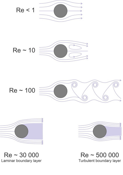
| Flow type | Wake characteristics | Drag level | |
|---|---|---|---|
| LAMINAR | Unseparated | Creeping flow | Low |
| \(\) | Separated | Separation bubbles | Moderate |
| \(\) | \(\) | Vortex street | Oscillating |
| \(\) | \(\) | Turbulent wake | Very high |
| TURBULENT | Separated | Narrower turbulent wake | High |
Now for our last example. We’ll return to the flat plate again, but this time turned through ninety degrees so it is aligned parallel to the oncoming flow. A flat plate arranged parallel to the flow leaves practically no wake at all, nor would you expect it to. The boundary layer doesn’t separate, and in any case there is no ‘upstream face’ or ‘downstream face’ for a normal pressure to act on. In this sense, a flat plate is an exemplar or model for any ultra-streamlined object such as stabilising fin, whose drag is largely caused by friction.
These three examples suggest how different kinds of vehicle might interact with the air or water through which they move. The first (a flat plate at right-angles to the undisturbed fluid stream) demonstrates that a sharp projection such as a wing mirror on an automobile can gouge out a disproportionately broad wake. It therefore produces a significant form drag. The third example shows that if a flat plate is aligned parallel to the flow as is approximately the case with a stabilising fin, the form drag almost disappears while friction drag takes centre stage. The second example, a circular cylinder, represents an intermediate class of body shapes that are not particularly well streamlined. Here, the pattern of motion within the wake varies with the vehicle speed.
The examples also demonstrate how a turbulent boundary layer can be turned to advantage, at least for bluff bodies like cylinders and motor cars. Remembering that it delays the point of separation, a turbulent boundary layer implies a narrower wake and less form drag. The down side is that a turbulent boundary layer exerts a greater friction drag than a laminar one, so it won’t help with a long, narrow body like an ocean liner or an aircraft wing where the friction acts over a large area. But it does help with more rounded shapes, a fact first brought to notice by Gustav Eiffel, the world-famous engineer who designed the Eiffel tower and was himself a gifted researcher in the field of hydrodynamics. Having built his own laboratory, among other things he showed that the drag acting on a sphere roughly halves above a speed corresponding to Re \(\sim\) 300 000. This happens to be the level at which the boundary layer switches from laminar to turbulent flow [2], and it explains why golf balls today have dimples moulded into their surface to ‘trip’ the fluid particles into turbulence as early as possible during their journey around the surface. In Section F1817 we’ll return to this topic in connection with moving vehicles.
Summary
Two hundred years ago, scientists treated a fluid as a very elusive substance: incompressible and friction-free. By doing so, they could predict its behaviour near a moving body, following a coherent pattern of streamlines that curved around the body profile. They could also predict the pressures that it exerted on the body surface, high in some places and low in others. But the pressures didn’t add up, or rather, they added up to nothing at all. The theory couldn’t explain resistance or drag, nor for that matter, could it explain the ‘lift’ provided by a bird’s wing. The missing factor was fluid viscosity, and there gradually emerged a more realistic theory that took viscosity into account through a radical concept: the boundary layer. In this Section we have seen how fluid particles stick to the body surface to create a slow-moving boundary layer that applies a shear force to the moving body and slows it down. At high speeds the boundary layer is flattened against the body surface, and the intense velocity gradient creates turbulence among the fluid particles; when it reaches a critical level, the transition from laminar to turbulent flow is signalled by a dimensionless parameter known as the Reynolds number. Like a litmus test, this parameter measures the relative importance of of viscous forces within the fluid mass, and has many applications throughout the field of fluid mechanics. We’ll tackle the fluid forces in more depth later in Section F1817. In the next Section, however, we’ll turn to a special kind of particle motion: the ‘free vortex’. Vortices occur in fluid motion on every physical scale ranging from microscopic eddies in your kitchen sink to the formation of galaxies in distant parts of the universe.
Appendix: The Navier-Stokes equations
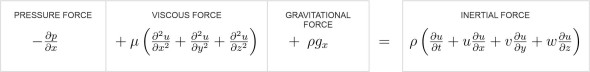
In 1822, the French engineer and physicist Claude-Louis Navier formulated a set of equations that were derived independently a few years later by George Stokes, who set them out in the form commonly found in textbooks today. Known as the Navier-Stokes equations, they represent Newton’s Second Law (force equals mass times acceleration) applied to a fluid element in the shape of a rectangular block [17]. The fluid is assumed to be an incompressible fluid with constant viscosity in steady laminar flow, and since the fluid is Newtonian, the shear stress acting on any given face is proportional to the strain rate. The particle momentarily occupies a rectangular box fixed in three-dimensional space, its edges being aligned with the \(x\), \(y\) and \(z\) axes of an orthogonal Cartesian coordinate system. The edges have dimensions \(\delta x\), \(\delta y\) and \(\delta z\). There are three separate equations. The first deals with the force components and the resulting acceleration component all of which act in the direction parallel to the \(x\)-axis, the second with the force components and acceleration acting parallel to the \(y\)-axis, and the third similarly in relation to the \(z\)-axis:
(19)
\[\begin{equation} -\frac{\partial p}{\partial x} + \mu \left( \frac{\partial^{2}u}{\partial x^2} + \frac{\partial^{2} u}{ \partial y^2 } + \frac{ \partial^{2} u }{ \partial z^2 } \right) + \rho g_{x} \quad = \quad \rho \left( \frac{\partial u}{\partial t} + u\frac{\partial u}{\partial x} + v\frac{\partial u}{\partial y} + w\frac{\partial u}{\partial z} \right) \end{equation}\](20)
\[\begin{equation} -\frac{\partial p}{\partial y} + \mu \left( \frac{\partial^{2}v}{\partial x^2} + \frac{\partial^{2} v}{ \partial y^2 } + \frac{ \partial^{2} v }{ \partial z^2 } \right) + \rho g_{y} \quad = \quad \rho \left( \frac{\partial v}{\partial t} + u\frac{\partial v}{\partial x} + v\frac{\partial v}{\partial y} + w\frac{\partial v}{\partial z} \right) \end{equation}\](21)
\[\begin{equation} -\frac{\partial p}{\partial z} + \mu \left( \frac{\partial^{2}w}{\partial x^2} + \frac{\partial^{2} w}{ \partial y^2 } + \frac{ \partial^{2} w }{ \partial z^2 } \right) + \rho g_{z} \quad = \quad \rho \left( \frac{\partial w}{\partial t} + u\frac{\partial w}{\partial x} + v\frac{\partial w}{\partial y} + w\frac{\partial w}{\partial z} \right) \end{equation}\]where
- \(p\) is fluid pressure,
- \(\mu\) is the dynamic viscosity of the fluid,
- \(\rho\) is the fluid density,
- \(t\) is time,
- \(x\), \(y\) and \(z\) are distances measured along the Cartesian axes,
- \(u\), \(v\), and \(w\) are the fluid velocities in the \(x\), \(y\) and \(z\) directions, and
- \(g_x\), \(g_y\), and \(g_z\) are the components of gravitational acceleration in the \(x\), \(y\), and \(z\) directions.
You can see where the various terms come from by referring to the derivation of the Euler equations in Section F1918, except that the viscous shear terms on the left-hand side don’t appear in the latter equations. The different terms represent different kinds of force at work within the fluid. Take, for example, equation 19. As shown in figure 25, the first term on the left hand side represents the component of the pressure force acting in the \(x\)-direction. The second and third terms represent the components of the viscous shear force and the gravitational force, again acting in the \(x\)-direction. The single term on the right hand side is just the mass of the block multiplied by the fluid acceleration in the \(x\)-direction, on the assumption that the block has unit volume. Text books often refer to the last term on the right as the ‘inertia force’, which is confusing because it is not a separate kind of force, but rather, it represents the outcome of all the forces acting on the block in terms of the particle’s acceleration. Other versions of the Navier-Stokes equations can be found that allow for unsteady, compressible flow [3] and for varying viscosity [5].
Figure 25