F.2019
Moving fluids
For centuries, scientists have studied the way things move, objects like cannon balls, vehicles, and planets in the solar system, all of which are essentially rigid and compact in nature. At any given moment, such an object has a precise location and a well-defined velocity, so you can work out its direction of motion and predict where it will be in a few seconds’ time, or maybe several hundred years in the case of a planet. But not everything can be treated in this way. Much of our environment is fluid in nature, like the atmosphere for example. Although we can feel the wind blowing in our faces, we can’t see the individual ‘particles’ of air and find it hard to judge their direction of motion. Water is another elusive substance: we can’t track individual particles as they move downstream because we can’t see them – what we see is a continuous flow. In some places the flow is smooth and steady, but in others it’s turbulent, with whirls and eddies that form on different scales of measurement, appearing and disappearing apparently at random, too quickly for us to follow.
Aspects of fluid motion
One of the aims of fluid mechanics is to predict what gases and liquids will do in different situations, for example, when water divides around a ship’s hull. We call the area we are looking at a flow field, and in the case of a moving vehicle, fluid will normally travel though it in a horizontal rather than a vertical direction. It’s conventional to draw it moving from left to right, although sometimes we’ll picture it the other way round. (In the case of a moving vehicle, it is really the vehicle that moves while the fluid stays more-or-less in place, but the result is essentially the same.) To understand what is happening one must track the progress of individual elements within the fluid mass - for brevity we’ll call them particles, although each ‘particle’ will contain millions of fluid molecules.
Streamlines and stream-tubes
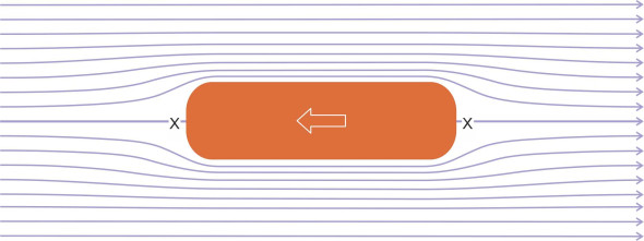
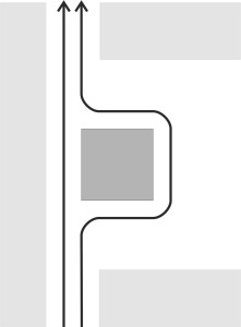
For much of the time we’ll be looking at situations where the flow is smooth and steady, so that if we focus on any particular location, neither the speed at which the particles are moving nor the direction of movement change over time. Also we’ll assume the fluid doesn’t undergo compression, as is usually the case for vehicles moving at subsonic speeds. It is often sufficient to picture the motion in two dimensions. For example, the movement of water above and below a hydrofoil blade follows broadly the same pattern at every point along the blade, so we need only to look at a typical cross-section to understand what is going on. In smooth flow, there are usually no empty spaces or cavities in the fluid, so that although neighbouring particles follow paths that may differ in curvature, their paths don’t cross over. This kind of movement can be represented by streamlines as shown in figure 1. Notice that the gap between neighbouring streamlines rises and falls from place to place across the flow field. The particles must speed up when the lines get closer together and slow down when they diverge so that the flow – the volume of fluid per unit time - remains constant. Since a particle won’t accelerate unless it’s pushed, wherever the streamlines converge the pressure must fall in the direction of flow to supply the motive force. Conversely, where the streamlines diverge the particles need a rising pressure gradient to make them slow down. In fact at certain points as indicated by the letter ‘X’ in figure 1, the particles may come to a halt. These are stagnation points, and they mark the places where the pressure is highest, typically at the nose and possibly the tail of a body moving through the fluid.
Figure 1
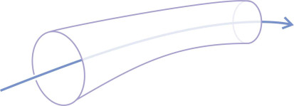
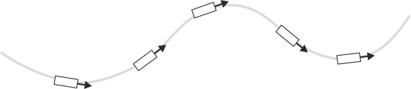
Most flow fields are really three-dimensional, and in principle we can extend the concept of a streamline to its 3D equivalent, the stream tube. A stream tube is an imaginary pipe through which particles flow without penetrating the walls, so the rate of flow is the same everywhere along the tube (figure 2). In theory, by bundling stream tubes together one can picture more complex patterns of flow in 3D space, but this doesn’t always work well on a computer screen.
Figure 2
Circulation
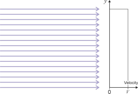
From here on we’ll confine our attention to 2D flow patterns, using streamlines to show how the fluid particles move within the flow field. There are many conceivable patterns of motion, but the simplest is one in which the particles all follow a straight line. Straight-line motion is easy to define for a moving vehicle like an aircraft: the different parts are rigidly connected so if we know the speed and direction of the fuselage we know straight away what the wings and tail are doing. A fluid is more complicated. Different particles can move at different speeds in different directions, so to define the equivalent of straight-line motion we need to specify that all the particles are moving in the same direction at the same speed, which implies that the streamlines are parallel and equally spaced as shown in figure 3. This pattern of motion is called a uniform flow field. It is a useful tool as we’ll see later in Section F1919.
Figure 3
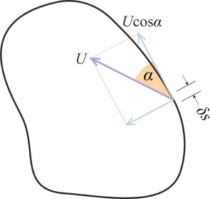
However, when fluid particles encounter a vehicle, the streamlines must divert around the body surface. If you turn back to figure 1 you’ll see the pattern of motion around a body depicted in plan view. It could be a bus. Since the body is symmetrical about its longitudinal axis, there’s no reason to suppose that the fluid might push it to one side or the other. But we know that a transverse force could arise if the body were asymmetrical. Imagine, for example, a ship in plan view. When the rudder swings to one side, fluid forces will push the stern in the opposite direction and cause the vessel to turn. Transverse forces of this kind are linked to a process called circulation. The idea is that the fluid motion around the body is biased either in a clockwise or an anticlockwise direction. The bias is defined in a specific manner, and it occurs whether or not a vehicle or indeed any other object is present. Imagine a closed loop C drawn around any region of a flow field. Individual streamlines may cross the curve or touch it at various points. At each point, the flow will have a component of velocity normal to the curve, and a tangential component as shown in figure 4. The tangential component measures the tendency for particles to orbit around the centre of the loop as opposed to moving radially towards or away from the centre. Let’s look at a particular streamline where it crosses the curve. If the velocity of fluid motion along the streamline is \(U\) and it crosses at an angle \(\alpha\) to the tangent as shown in the Figure, the tangential component is \(U \cos \alpha\). If the streamline touches the curve but doesn’t cross it, we take \(\alpha\) as being zero so that \(\cos \alpha = 1\) and the tangential component is just \(U\). By summing the tangential components of all the streamlines that cross or touch the curve you arrive at a quantity known as the circulation \(\Gamma\), given by
(1)
\[\begin{equation} \Gamma \quad = \quad \oint \left(U \cos \alpha \right) ds \end{equation}\]where the symbol \(\oint\) indicates integration along successive elements of the curve each of length ds. If we were to calculate the value of \(\Gamma\), what would it tell us? A non-zero value doesn’t necessarily imply that the fluid particles are actually travelling in circles, only that their paths are biased either in a clockwise direction or an anticlockwise direction according to the sign of \(\Gamma\). By convention, an anti-clockwise circulation is taken as positive for most applications other than aircraft flight, where it’s the other way round.
Figure 4
To understand what this means, think of a crowd entering a railway station during the morning rush hour. Inside the station entrance is a kiosk with its counter facing to the right, its four walls forming a square of side \(s\). In figure 5 we see the stream of travellers entering the station and dividing around either side of the kiosk. They are all heading for the departure platforms beyond, and walking at the same speed. No-one stops or makes a complete circle around the kiosk. This doesn’t mean the circulation \(\Gamma\) is zero. There is a bias, a preponderance of movement in a particular direction. If we take the four walls of the kiosk as defining our ‘loop’, then the angle \(\alpha\) at which the people are moving relative to each wall is zero and \(\cos \alpha = 1\) everywhere around the loop. For each wall of the kiosk we can work out separately the contribution to the overall circulation made by the pedestrians moving along that wall; it is equal to the speed \(U\) times \(\cos \alpha\) times the length \(s\) of that wall, which is just \(Us\) (note that for the purposes of this exercise, the number of pedestrians passing along either side of the kiosk is irrelevant - we are concerned only with their speed of motion). For the left-hand wall the motion is clockwise so by convention its contribution is negative, while for the other three it is anticlockwise and therefore positive. Overall, \(\Gamma\) comes to \(- Us + 3Us = 2Us\), in other words, there is a net anticlockwise circulation. A bias could arise in a different way if the commuters walked, for example, more slowly around the right-hand side of the kiosk in order to look at the magazines on display. If they walked slowly enough, the circulation could even change sign. As we’ll see in Section A2020, the concept of circulation turns out to be useful for understanding the lift generated by an aircraft wing.
Figure 5
Rotation
When people move around on foot, they usually face the way they are going, otherwise they are likely to bump into something or fall over. Machines likewise. The orientation of a railway locomotive is locked to the direction of motion, with the cab facing forward along the track (figure 6). If the track curves to the right, the locomotive will follow the curve and simultaneously rotate so that it points in the direction it is going.
Figure 6
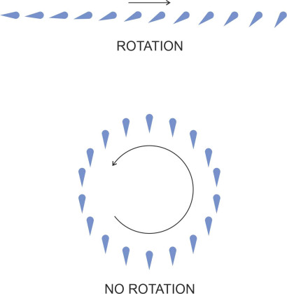
But a fluid particle is different. Its orientation is not locked to the streamline that it follows. It behaves more like a helicopter, which can rotate independently if the pilot wants it to. The upper diagram of figure 7 shows the pilot steering along a straight line while rotating the fuselage steadily anticlockwise. In the lower diagram, the pilot circles around an airfield while keeping the fuselage pointing in a fixed direction, north, so the helicopter follows a circular path without rotating at all.
Figure 7
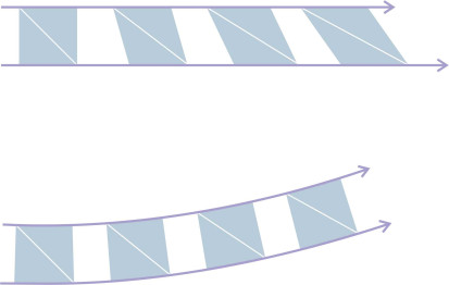
In the case of fluid particles, however, there’s a difference: there is no-one at the controls. A particle has inertia and under normal circumstances it cannot rotate unless a torque is applied to it by its neighbours: there must be viscous friction, and to bring this friction to bear, the particles on one side must be moving faster than those on the other. In other words, there must be a velocity gradient across the streamlines. In the upper diagram of figure 8 we see a particle travelling in a straight line. The particles in the layer immediately below are moving faster than those in the layer immediately above, and the rectangular chunk of fluid highlighted in blue distorts as it moves across the flow field. The change in alignment of the white diagonal shows in fact that it is rotating anticlockwise during the process. In the lower diagram the particle travels in a circular orbit; it keeps the same shape throughout, but it’s rotating anticlockwise here too.
Figure 8
The intensity of rotation is measured by a quantity called the vorticity, denoted by \(\xi\). For an infinitesimally small area within a two-dimensional flow field in the \(x\), \(y\) plane, it is equal to the circulation per unit area and it is defined by
(2)
\[\begin{equation} \xi \quad = \quad \frac{\partial v}{\partial x}-\frac{\partial u}{\partial y} \end{equation}\]where \(u\) is the velocity component parallel to the \(x\)-axis and \(v\) is the velocity component parallel to the \(y\)-axis. It is a point property, meaning that it varies from place to place in the flow field. Vorticity is a theoretical construct rather than a tool that aerodynamicists use in the design office, but it represents the final link in a chain of three related concepts that together have a very practical bearing on the hydrodynamics of moving vehicles:
- Viscosity: all fluids possess some degree of viscosity but in some cases – for example, air and water - the viscosity is small.
- Rotation: the category of motion that is unique to fluids. Each fluid particle has inertia, and without viscosity, there can be no friction between the particle and its neighbours, and no force to make it rotate (and curiously, if by some magical intervention rotation were already present, it couldn’t be undone).
- Vorticity: the numerical quantity that measures the degree of rotation.
Later in this web site, we’ll look more closely at viscous fluids and try to make sense of their behaviour. In this Section and the two Sections that follow, we’ll suppose that the fluid has zero viscosity and explore the consequences. For an inviscid fluid the vorticity is zero throughout and the flow is said to be irrotational. Although this doesn’t seem a very realistic scenario, the results turn out to be surprisingly useful, for two reasons. First, the assumption of zero viscosity greatly simplifies the mathematics, and second, most vehicles move through air and water, whose viscosity is sufficiently small that the fluid behaves as if it were irrotational anyway, at least throughout much of the flow field.
Figure 9
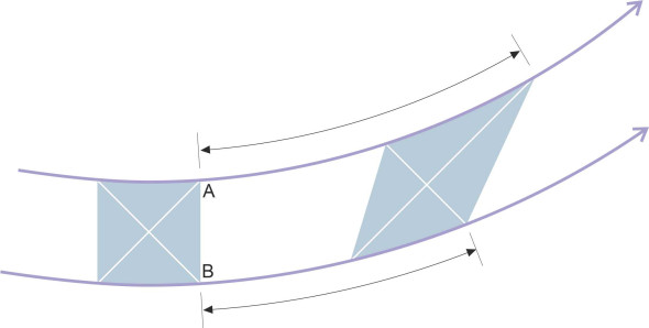
However, the fluid particles will change shape whenever they move round a curve. In figure 9 we see a chunk of non-viscous fluid moving along an arc. At the start of the sequence, the outline shape of the chunk is roughly square when viewed from the side. There are normal pressures acting on all four sides but no shear forces. As the chunk moves from left to right, it can’t rotate so the alignment of the diagonals doesn’t change. But the outline is squeezed into a diamond shape, which makes something else happen as well. Let’s focus on the two leading corners marked A and B. By the time it reaches the right-hand edge of the diagram, the inside corner A has moved considerably further than the outside one. This is not an artefact, but an inescapable consequence of being squeezed without rotating - particles on the inside of a curve will move faster than those on the outside. As will emerge later in Section F1919, for irrotational flow there is a simple relationship between the path radius r and the velocity U along a streamline:
(3)
\[\begin{equation} U \quad \propto \quad \frac{1}{r} \end{equation}\]Figure 10
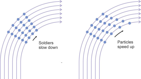
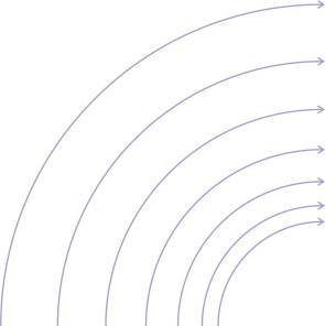
This might seem odd, indeed the opposite of what you’d expect. As shown in figure 10, when soldiers march in formation and they turn to the right or to the left, those on the inside of the curve slow down so that the formation keeps its shape. But fluids don’t keep their shape, and here, we are predicting the fluid particles on the inside of a curve will move faster. The smaller the radius, the faster they travel, and towards the centre of curvature, the velocity increases without limit! To a reasonably close approximation, fluids with modest viscosity such as air and water do in fact behave like this, and as shown in figure 11, the gaps between the streamlines fall progressively with decreasing radius. At this point, it seems natural to wonder what would happen if the ends of the path were joined together to form a closed loop? The result is a whirling flow pattern known as a vortex.
Figure 11
Vortices
Vortices occur naturally on different physical scales. On the largest scale are the weather systems that develop over tropical seas: hurricanes and typhoons in which the wind spirals with increasing force towards the centre of the system from an area several hundred kilometres across, drawn by a column of air rising from the ‘eye’ of the storm. A weather system of this kind may persist for several weeks. On a smaller scale are the vortices that occur in a river as it flows around obstacles, or wind blowing over an irregular landscape. Often described as whirls and eddies, they are triggered by abrupt changes in the ground surface, or the river bed beneath. Finally on the smallest physical scale are the fleeting, irregular vortices that characterise turbulence.
The different types of vortex behave in different ways, and not all follow a steady or consistent pattern of movement. But there are two cases that can be described more-or-less accurately by a theoretical model. The first happens when you spin a bucket of water on a turntable. The body of water inside the bucket has a roughly cylindrical shape. At first it will resist motion because of its inertia, appearing to remain stationary while the bucket revolves around it. However, friction with the bucket causes the outer layer of fluid to accelerate, and gradually, this movement is propagated to the inner layers until the whole body of liquid reaches the same angular velocity as the container, spinning as if it were a solid mass. The resulting pattern is called a forced vortex and it has a distinguishing feature: the particles towards the outside move faster than those close to the centre, where the fluid velocity is zero. The second case is the one more often found in nature, the free vortex. It occurs in fluids of low viscosity like air and water, and the pattern of motion more closely resembles that of an irrotational fluid. For such a fluid, the velocity at any particular radius \(r\) is inversely proportional to \(r\), and the consequences are startling. In theory as one gets close to the centre, the particles move at increasing speed – theoretically infinite - with no obvious driving force, a situation as different from a forced vortex as it is possible to imagine. These two cases describe ideal situations at either end of a spectrum while real vortices usually lie somewhere between. It is fascinating to experiment with water in your kitchen sink, by adding a few drops of dishwasher liquid until bubbles appear on the surface. When the contents have settled, dip a serving spoon vertically into the fluid and draw it slowly across from one side to the other. If you’re lucky, one or more eddies will appear as if propelled by gears that somehow magnify the speed of rotation.
From a practical point of view, vortices are important because among other things, they affect the way vehicles move. For example, circulatory motion around the wings of an aircraft enables them to generate lift, while vortices shed from the wingtips can de-stabilise other aircraft following behind along the same flight path. In the case of road vehicles, vortices cause drag by carrying off energy, and even affect handling behaviour. These are topics we’ll take up later in Section F1818 and elsewhere.
Turbulence
Ealier we mentioned that a fluid flow might be ‘turbulent’. It’s an important distinction. Many vehicles have slender bodies whose rounded surfaces cause minimal disturbance to the surrounding fluid when travelling at low speeds. When displaced around the body surface, each fluid particle follows a smooth trajectory that is almost parallel to those of its neighbours, their paths arranged in a geometrical pattern that remains stable over time. Motion of this kind is called laminar flow. As the speed rises, at a critical point the flow pattern will change. The motion becomes erratic, with waves and eddies forming initially on a microscopic scale. The streamlines now represent ‘average’ motion. Particles will cross them at random and inter-mix with those in the neighbouring layers, which effectively increases the level of viscosity and with it, the level of friction ‘drag’ that tends to slow the vehicle down. Motion of this kind is called turbulent flow. For transport vehicles travelling at normal cruising speed, the flow around the body surface is usually turbulent, and inside the wake, eddies may occur on a larger scale. Later in Section F1917 we’ll return to this topic in more detail.
Categories of flow
A fluid can behave in different ways according to the circumstances. Our challenge is to understand its behaviour and predict its effects on a vehicle passing through the flow field. To simplify the problem, scientists have identified (a) certain characteristics of fluid motion, and (b) certain properties of the fluid itself, that play a central role. In principle, the presence or absence of any one of them may be relevant to the problem at hand. They can occur singly or in combination, and at this point it may be helpful to recap the ones we have met so far, and pick out the combinations that typically arise in connection with moving vehicles.
Towards a basic classification
The most important characteristics are listed in table 1. They are set out in pairs, as mutually exclusive alternative states. For example, a flow might be viscous or it might be inviscid, but we don’t allow for anything in between. So we can classify our flow by working through the table and choosing one of the two alternative states from each row. There are \(2^{5}\) different ways in which this can be done, implying that there are potentially 32 different kinds of fluid flow, but in reality most of the combinations can be ruled out. For example, a non-continuum flow of gas molecules can’t be viscous because by definition, the molecules don’t interact. Nor can an inviscid flow be turbulent, because eddies can’t form in a frictionless medium.
| Potential characteristics |
|---|
| Continuum / non-continuum |
| Viscous / inviscid |
| Rotational / irrotational |
| Laminar / turbulent |
| Compressible / incompressible |
So where does that leave us? By convention, engineers and scientists distinguish only two basic categories of fluid: Ideal and Newtonian. Both behave in the way you would expect a continuous medium to behave, and both have properties that match (or approximately match) flows that we observe in everyday life, in particular those associated with moving vehicles. The motion of an Ideal fluid is always laminar, while Newtonian fluid flow can be laminar or turbulent. Both are continuum flows that don’t involve significant compression. We’ll describe these two flow categories in more detail shortly, and then turn briefly to compressible flow. Non-continuum flows and compressible flows are usually treated as separate genres each requiring a distinctive mathematical approach.
Ideal fluid
An ideal fluid doesn’t exist. It’s a theoretical model that makes fluid behaviour easier to analyse. Try to imagine a slippery substance that would be impossible to grasp, feel, or hold in your hands unless confined in a container. Inviscid and irrotational, it’s usually assumed to be incompressible too, so you can’t squeeze it into a smaller space, or for that matter, stretch it out into a larger one. The fundamental equations that describe the movement of such a fluid were formulated during the mid-eighteenth century by Leonhard Euler (1707-1783) and developed by Lagrange and Laplace into the form we know today. They can be solved to predict the pattern of flow around a streamlined shape. However, being friction-free, an ideal fluid can’t exert a shear force on a vehicle body, and while it can apply a normal pressure at right angles to the body surface, as we’ll try to explain in later Sections, the resultant force on the vehicle is always zero. To handle forces such as a ‘lift’ and ‘drag’, we need a model that includes friction.
Newtonian fluid
The second fundamental fluid category is the Newtonian fluid. It is a more realistic representation of a real gas or liquid because it is viscous, and as specified earlier in the previous Section, the coefficient of viscosity \(\mu\) is constant, so the shear force is proportional to the velocity gradient. Analysing the motion of a Newtonian fluid is an order of magnitude more difficult than analysing the motion of an ideal fluid, but there are two ways to go about it. One of them is to simulate the motion on a computer. The other is much older, and involves equations that were formulated during the 19th century and are now referred to as the Navier-Stokes equations. Although they are difficult to solve, about 100 years ago, scientists and mathematicians made a breakthrough. They had spent a great deal of time and effort trying to understand the flow over an aircraft wing, in which the particles close to the wing surface are slowed down by viscous friction. During the 1920s, led by the brilliant engineer/scientist Ludwig Prandtl, they realised that since the influence of viscosity was confined to a thin layer, the flow field could be broken down into two parts: the non-viscous outer part, and the viscous boundary layer. The two-dimensional geometry of the boundary layer enabled the flow pattern to be modelled locally using a simplified version of the Navier-Stokes equations, so that investigators could work out expressions for the friction drag and ultimately design efficient wing profiles.
Compressible flow
‘Compressible flow’ is a sub-category of motion in which the density of the fluid (which can be either an ideal fluid or a Newtonian fluid) is allowed to rise or fall in reponse to pressure variations as it moves across the flow field. It occurs frequently in connection with aircraft travelling at high speed, and also inside steam turbines – it was a problem with naval vessels before military aircraft appeared on the scene.
The ability to undergo compression and dilation makes makes the analysis of fluid motion more complicated. To understand why, it will help us to examine how disturbances in a fluid propagate from place to place (a) in an incompressible fluid, and (b) in a compressible one. Let’s start with case (a). Imagine an alternative universe in which the earth’s atmosphere is incompressible. Early one morning, you are standing outside a bus depot in West London. All is quiet. Suddenly the door opens, a horn blares, and a bus shoots out of the depot. What is happening to the air in its path? According to classical fluid mechanics, the front of the bus applies pressure to the particles so they move out of the way. The pressure changes are propagated from one particle to the next, and since the air can’t be compressed the effect is immediate. If you look at figure 1, which shows the bus from above, you can see the streamlines dividing some distance ahead of the vehicle. They’re at a slight angle to the bus centreline, and this angle signifies a pressure change propagated ahead of the vehicle that causes the fluid particles to alter their speed and direction of motion. Looking along the intended path of the bus, how far ahead does this influence extend? The answer is determined by the shapes of the streamlines, and the mathematics tells us that the streamlines are diverging for as far ahead as you care to look. Hence there’s no time lag: the air begins to move as soon as the bus emerges from the depot. If the passengers waiting at Heathrow were sensitive to disturbances in the atmosphere, they would know immediately that a bus was on its way. And in this alternative universe, so would passengers in New York.
You might find this a little implausible, and you’d be right. An incompressible fluid is a convenient fiction: it simplifies analysis but it contravenes the laws of physics. No physical disturbance can propagate instantaneously across the Atlantic Ocean. In reality, the air is compressible and the disturbance moves ahead of the bus at a finite speed – the speed of sound in air, about 1227 km/h at sea level, and the bus’s departure would take more than 15 seconds to register at Heathrow airport. And this brings us to another question: what would happen if the bus were to accelerate until it reached the speed of sound? The answer is that it would catch up with its own disturbance, which wouldn’t propagate fast enough to get out of the way. The particles would pile up against the vehicle nose, creating a shock wave and a sonic ‘boom’. The pressure and density increase abruptly when air passes through a shock wave, which is paper-thin. The temperature rises too, because some of the particle momentum is dissipated as heat.
To account for this behaviour, compressible flow requires a different kind of mathematical model from the ones normally applied to fluid motion. The streamlines follow a different pattern and there are two new variables involved, namely density and temperature. In later Sections we’ll see how the shape and size vary of a shock wave varies according to the speed of flow, and how the speed of flow itself varies from place to place over the aircraft body surface. Shock waves imply extra drag, and if the body is moving at hypersonic speed (five times faster than the speed of sound), the air passing through a shock wave may reach a temperature higher than the melting point of steel.
Conclusion
By now you’ll be getting the idea that fluid flow is a tricky problem. It has challenged the capabilities of researchers for two centuries and continues to do so today [1] [3] [4] [5] [6] [7]. As the historian Olivier Darrigol put it: ‘What distinguishes the history of hydrodynamics is the slowness with which \(\ldots\) (the) challenges were met’ [2]. Of the Sections that follow in this part of the web site, many are devoted to explaining the difficulties. We’ll see how engineers, scientists and mathematicians have found ways of predicting the flow of air and water around moving vehicles, and in particular, the forces they exert on the body surface.