F.1918
Bernoulli’s equation
The pipe that brings water into your home is a beautifully simple device: a rod with a hole right through the middle. Water is pumped into one end, it travels along the pipe, and it pours out at the other end into your kitchen sink. It may look simple, but historically, the development of the supply system was a significant technical achievement. It began to take shape in Europe during the 18th century, when manufacturers discovered how to make pipes cheaply enough for water to be ducted underground on a large scale. However, not all schemes worked, at least not very well, and many years passed before scientists and engineers discovered how water behaves when moving in a confined space (or, for that matter, in any kind of flow field). What happens, for example, when the water particles pass from a broad channel into a narrower one, or from a pipe of large cross-section into a smaller one? Intuitively, you’d think the particles would slow down, but as we saw in the last Section, they speed up. They have to, in order to sustain the same rate of flow at all points along the pipe. A more surprising discovery was what happens to the pressure between the particles at the point where the pipe narrows. We humans feel uncomfortable when we join the crowd entering a narrow passageway in a busy underground station - the pressure of bodies around us seems to rise. With a fluid, what happens is almost exactly the opposite: the pressure falls. Although the 18th century engineers were aware of this, no-one understood why it happened until Daniel Bernoulli (1700 – 1782) began to put fluid mechanics on a systematic footing. In 1738 he published his great work Hydrodynamica, in which he observed that fluid velocity and pressure are connected through a ‘see-saw’ relationship – when one rises the other falls. This observation led to a mathematical equation that we now call Bernoulli’s Law, perhaps the most widely used ‘law’ in fluid mechanics. In fact, the equation can take different forms, and Bernoulli himself wasn’t responsible for any of them.
Derivation
We’ve already seen in Section F1919 how the speed at which fluid particles move varies from place to place within the flow field. The pressure varies too, and to understand the pressure variations we have to think about what happens on the microscopic scale. It was Bernoulli’s pupil Leonhard Euler (1707-1783) who conceived the mathematical framework that is needed to answer questions of this kind. He pictured the flow field as an assembly of small elements each shaped like a rectangular block whose position was fixed in three-dimensional space. The idea was to reconcile the motion of the fluid in each element with that of its neighbours, focussing on the acceleration arising from all the forces at work assuming that the mass of fluid within the element obeyed Newton’s second law. Any fluid element is pushed and pulled by an array of forces, and responds by changing velocity. If it’s a non-viscous fluid, there are no shear forces, only normal forces acting on each of the six faces of the element. If it’s a viscous fluid, there will be shear forces as well. The mathematics looks forbidding, but we’ll describe the derivation of Bernoulli’s Law in detail, if only to give you some idea of the challenge that the 18th century physicists and mathematicians were facing. There was no established notation, and few knew what a differential equation was, let alone how to solve it. At least the underlying principles are straightforward.
| Variable | Meaning |
|---|---|
| \(x\), \(y\) and \(z\) | Distances measured along the axes of an orthogonal coordinate system |
| \(\rho\) | Fluid density |
| \(g_{x}\) | Component of acceleration due to gravity acting parallel to the \(x\)-axis |
| \(\tau_{xy}\) | Shear stress acting on face ‘X’ normal to the \(x\)-axis parallel to the \(y\)-axis |
| \(\tau_{xz}\) | Shear stress acting on face ‘X’ normal to the \(x\)-axis parallel to the \(z\)-axis |
| \(\tau_{yx}\) | Shear stress acting on face ‘Y’ normal to the \(y\)-axis parallel to the \(x\)-axis |
| \(\tau_{yz}\) | Shear stress acting on face ‘Y’ normal to the \(y\)-axis parallel to the \(z\)-axis |
| \(\tau_{zx}\) | Shear stress acting on face ‘Z’ normal to the \(z\)-axis parallel to the \(x\)-axis |
| \(\tau_{zy}\) | Shear stress acting on face ‘Z’ normal to the \(z\)-axis parallel to the \(y\)-axis |
| \(\sigma_{xx}\) | Normal stress on face ‘X’ normal to the \(x\)-axis |
| \(\sigma_{yy}\) | Normal stress on face ‘Y’ normal to the \(y\)-axis |
| \(\sigma_{zz}\) | Normal stress on face ‘Z’ normal to the \(z\)-axis |
| \(u\), \(v\), \(w\) | Velocities in direction of \(x\), \(y\) and \(z\) axes respectively |
| \(t\) | Time |
Figure 1
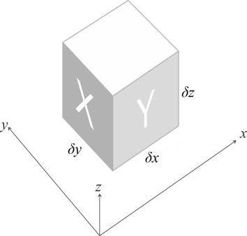
Euler’s equations of motion
Each fluid element occupies an infinitesimally small rectangular box located in three-dimensional space as shown in figure 1. The three faces closest to the origin are labelled ‘X’, ‘Y’ and ‘Z’ but the ‘Z’ face is underneath and not visible in the Figure. Measured parallel to the axes, the sides are of length \(\delta x\), \(\delta y\) and \(\delta z\). The fluid density is \(\rho\), which may or may not be fixed. At any given time \(t\), the fluid inside the box is moving with velocity components \(u\), \(v\), and \(w\) respectively in the \(x\), \(y\) and \(z\)-directions. The stresses acting on the fluid are shown in figure 2; we follow the notation used by [6], which is reproduced in table 1 so you can keep track (if you want to). Notice that the stresses act in opposite directions on opposite faces, but they don’t quite cancel out. For example, the normal stress \(\sigma_{xx}\) acting on the face coloured in darker grey changes to \(\sigma_{xx} + \delta x \left( \partial \sigma_{xx} / \partial x \right)\) at the opposite face. The Figure shows only the stresses that act in the x-direction; those acting in the y-direction and the z-direction follow a similar pattern.
Figure 2
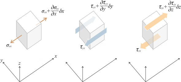
The next step is to convert the stresses into forces. Force equals stress times area, so the normal stress \(\sigma_{xx}\) acting on the darker grey face produces a normal force of -\(\sigma_{xx} \delta y \delta z\) measured positive in the \(x\)-direction. Similarly the shear stress \(\tau_{yx}\) acting on the light grey face generates a force \(-\tau_{yx} \delta x \delta z\) measured positive in the \(x\)-direction. Summing over all six faces, we determine the overall force \(F_{Sx}\) due to surface stresses in the \(x\)-direction as being
\(F_{Sx} \quad =\quad \left[ \left( \sigma_{xx} + \frac{\partial \sigma_{xz}}{\partial x} \delta x \right) \delta y \delta z + \left( \tau _{yx} + \frac{\partial \tau _{yx}}{\partial y} \delta y \right) \delta x \delta z + \left( \tau _{zx} + \frac{\partial \tau _{zx}}{\partial z} \delta z \right) \delta x\ \delta y \right]\)\(- \left[ \sigma_{xx} \delta y \delta z + \tau _{yx} \delta x \delta z + \tau _{zx} \delta x \delta y \right]\)which simplifies to
(1)
\[\begin{equation} F_{Sx} \quad = \quad \left( \frac{\partial \sigma _{xz}}{\partial x} + \frac{\partial \tau _{yx}}{\partial y} + \frac{\partial \tau _{zx}}{\partial z} \right) \delta x \delta y \delta z \end{equation}\]There remains the weight of the fluid particle to be taken into account. We haven’t yet specified the orientation of the axis system so there could be a component \(g_{x}\) of the acceleration due to gravity acting in the \(x\)-direction, which implies a gravitational force \(F_{Gx}\) acting in that direction equal to the fluid density \(\rho\) times the volume \(\delta x \delta y \delta z\) times \(g_{x}\), or \(\rho g_{x} \delta x \delta y \delta z\). The total force \(F_{x}\) in the \(x\)-direction now becomes
(2)
\[\begin{eqnarray} F_{x} \quad & = & \quad F_{Sx} + F_{Gx} \nonumber \\ \nonumber \\ \nonumber & = & \quad \left( \frac{\partial \sigma_{xz}}{\partial x} + \frac{ \partial \tau_{yx}}{\partial y} + \frac{\partial \tau_{zx}}{\partial z} \right) \delta x \delta y \delta z + \rho g_{x} \delta x \delta y \delta z \nonumber \\ \nonumber \\ & = & \quad \left( \rho g_{x} + \frac{\partial \sigma_{xz}}{\partial x} + \frac{\partial \tau_{yx}}{\partial y} + \frac{\partial \tau_{zx}}{\partial z} \right) \delta x \delta y \delta z \end{eqnarray}\]To apply Newton’s Law we also need an expression for the acceleration. This is not as straightforward as it might seem. In the Eulerian description of a flow field, the velocity is a field. The speed of fluid passing through any element that fixed in three-dimensional space can change for two distinct reasons: (a) the flow may be unsteady, meaning that the velocity field is changing over time, or (b) the fluid is moving through a field in which the velocity changes with position. Both processes can take place simultaneously. An unsteady velocity field that is changing over time will give rise to an acceleration component \(\partial u / \partial t\). If in addition a fluid particle undergoes acceleration because its velocity is changing as it moves from place to place within the flow field, the component of its speed in the \(x\)-direction will change from \(u\) to \(u + \left( \partial u / \partial x \right).\delta x\) as it passes through the rectangular box; the speed difference is \(\left( \partial u / \partial x \right) . \delta x\) and the corresponding acceleration component is \(\left( \partial u / \partial x \right) . \left( \delta x/ \delta t \right)\) or \(u \left( \partial u / \partial x \right)\). Two other acceleration components (again in the \(x\)-direction) arise from the variations in \(u\) with motion in the other two directions \(y\) and \(z\), with the result that the overall acceleration \(a_{x}\) in the \(x\)-direction is
(3)
\[\begin{equation} a_{x} \quad = \quad \frac{\partial u}{\partial t} + u\frac{\partial u}{\partial x} + v\frac{\partial u}{\partial y} + w\frac{\partial u}{\partial z} \end{equation}\]Similar expressions can be constructed for the acceleration \(a_y\) in the \(y\)-direction and the acceleration \(a_{z}\) in the \(z\)-direction. Together, the three expressions constitute a vector that is technically known as the ‘material derivative’ (or alternatively the ‘substantial derivative’).
We’ll continue to focus attention on motion in the \(x\)-direction and apply Newton’s second law, putting the applied force \(F_{x}\) as equal to the mass \(\rho \delta x \delta y \delta\) of fluid in the box times the acceleration \(a_{x}\), to obtain
(4)
\[\begin{equation} F_{x} \quad = \quad \rho \delta x \delta y \delta z.a_{x} \end{equation}\]which on substituting the right-hand side of equation 2 for \(F_{x}\) and the right-hand side of equation 3 for \(a_x\) and cancelling the factor \(\delta x \delta y \delta z\) becomes:
(5)
\[\begin{equation} \rho g_{x} + \frac{\partial \sigma_{xx}}{\partial x} + \frac{\partial \tau_{yx}}{\partial y} + \frac{\partial \tau_{zx}}{\partial z} \quad = \quad \rho \left( \frac{\partial u}{\partial t} + u \frac{\partial u}{\partial x} + v \frac{\partial u}{\partial y} + w \frac{\partial u}{\partial z} \right) \end{equation}\]In a similar way, one can derive corresponding equations for motion in the \(y\)- and \(z\)-directions thus:
(6)
\[\begin{equation} \rho g_{y} + \frac{\partial \tau_{xy}}{\partial x} + \frac{\partial \sigma_{yy}}{\partial y} +\frac{\partial \tau_{zy}}{\partial z} \quad = \quad \rho \left( \frac{\partial v}{\partial t} + u\frac{\partial v}{\partial x} + v \frac{\partial v}{\partial y} + w\frac{\partial v}{\partial z} \right) \end{equation}\](7)
\[\begin{equation} \rho g_{z} + \frac{\partial \tau_{xz}}{\partial x} + \frac{\partial \tau_{yz}}{\partial y} + \frac{\partial \sigma_{zz}}{\partial z} \quad = \quad \rho \left( \frac{\partial w}{\partial t} + u\frac{\partial w}{\partial x} + v\frac{\partial w}{\partial y} + w\frac{\partial w}{\partial z} \right) \end{equation}\]The equations are unwieldy and experts usually express them in tensor notation. But we can simplify them for an inviscid fluid because all the shear stresses disappear, and furthermore the normal stresses \(\sigma_{xx}\), \(\sigma_{yy}\) and \(\sigma_{zz}\) are all numerically equal to the local pressure \(p\) but of opposite sign, so we get:
(8)
\[\begin{equation} \rho g_{x} - \frac{\partial p}{\partial x} \quad = \quad \rho \left( \frac{\partial u}{\partial t} + u\frac{\partial u}{\partial x} + v\frac{\partial u}{\partial y} + w\frac{\partial u}{\partial z} \right) \end{equation}\](9)
\[\begin{equation} \rho g_{y} - \frac{\partial p}{\partial y} \quad = \quad \rho \left( \frac{\partial v}{\partial t} + u\frac{\partial v}{\partial x} + v\frac{\partial v}{\partial y} + w\frac{\partial v}{\partial z} \right) \end{equation}\](10)
\[\begin{equation} \rho g_{z} - \frac{\partial p}{\partial z} \quad = \quad \rho \left( \frac{\partial w}{\partial t} + u\frac{\partial w}{\partial x} + v\frac{\partial w}{\partial y} + w\frac{\partial w}{\partial z} \right) \end{equation}\]Later we’ll simplify these equations further by assuming steady flow. But we are still left with a coupled system of non-linear partial differential equations for which there is no general solution; the non-linear terms are the ones like \(u \left(\partial u / \partial x \right)\) and \(v \left( \partial u / \partial y \right)\). Euler never solved them for any meaningful application. It was the mathematicians who followed him, Lagrange and Laplace, who re-cast them into a different form. We’ll work through an equivalent process here, following the steps as set out in [6], but expressed in conventional rather than vector notation. It’s hard going and there are easier ways to arrive at Bernoulli’s Law, but for reasons we’ll explain later, it’s worth the effort.
Deriving Bernoulli’s equation
To get to Bernoulli’s equation we first ensure that our frame of reference is aligned with the z-axis pointing vertically upwards. Then the acceleration due to gravity acts in the opposite direction, so we can write \(g_{z} = -g\), \(g_{x} = 0\), and \(g_{y} = 0\). Assuming steady flow, we have \(\partial u / \partial t = \partial v / \partial t = \partial w / \partial t = 0\); equations equation 8, equation 9 and equation 10 then simplify to
(11)
\[\begin{equation} - \frac{\partial p}{\partial x} \quad = \quad \rho \left( u \frac{\partial u}{\partial x} + v\frac{\partial u}{\partial y} + w\frac{\partial u}{\partial z} \right) \end{equation}\](12)
\[\begin{equation} - \frac{\partial p}{\partial y} \quad = \quad \rho \left( u \frac{\partial v}{\partial x} + v\frac{\partial v}{\partial y} + w\frac{\partial v}{\partial z} \right) \end{equation}\](13)
\[\begin{equation} - \rho g - \frac{\partial p}{\partial z} \quad = \quad \rho \left( u\frac{\partial w}{\partial x} + v \frac {\partial w}{\partial y} + w\frac{\partial w}{\partial z} \right) \end{equation}\]Now for a little mathematical sleight-of-hand. We’ll add two new terms to the right-hand side of equation 11 and arrange all the terms in a different order. The new terms are \(v \left ( \partial v /\partial x \right)\), and \(w \left( \partial w / \partial x \right)\), and they appear in the first set of braces on the right-hand side of equation 14 below. You’ll notice that we subtract them again in the second set of braces so nothing has materially changed:
(14)
\[\begin{equation} - \frac{\partial p}{\partial x} \quad = \quad \rho \left( u \frac{\partial u}{\partial x} + v \frac{\partial v}{\partial x} + w\frac{\partial w}{\partial x} \right)\ - \rho \left( v\frac{\partial v}{\partial x} - v \frac{\partial u}{\partial y} - w \frac{\partial u}{\partial z} + w \frac{\partial w}{\partial x} \right) \end{equation}\]Now, for irrotational flow the vorticity is zero so by definition:
(15)
\[\begin{equation} \xi_{x} \quad = \quad \frac{\partial w}{\partial y} - \frac{\partial v}{\partial z} \quad = \quad 0 \nonumber \end{equation}\](16)
\[\begin{equation} \xi_{y} \quad = \quad \frac{\partial u}{\partial z} - \frac{\partial w}{\partial x} \quad = \quad 0 \nonumber \end{equation}\](17)
\[\begin{equation} \xi_{z} \quad = \quad \frac{\partial v}{\partial x} - \frac{\partial u}{\partial y} \quad = \quad 0 \nonumber \end{equation}\]which means that the terms within the second set of braces on the right hand side of equation 14 add up to zero, and we now have
(18)
\[\begin{eqnarray} - \frac{\partial p}{\partial x} \quad & = & \quad \rho \left( u \frac{\partial u}{\partial x} + v \frac{\partial v}{\partial x} + w\frac{\partial w}{\partial x} \right)\nonumber \\ & = & \quad \rho \left[ \frac{1}{2}\frac{\partial \left( u^{2} \right)}{\partial x} + \frac{1}{2}\frac{\partial \left( v^{2} \right)}{\partial x} + \frac{1}{2}\frac{\partial \left(w^{2} \right)}{\partial x} \right] \nonumber \\ & = & \quad \frac{1}{2}\rho \frac{\partial }{\partial x} \left( u^{2} + v^{2} + w^{2} \right) \nonumber \end{eqnarray}\]and the right-hand side can be simplified to obtain the result:
(19)
\[\begin{equation} - \frac{\partial p}{\partial x} \quad = \quad \frac{1}{2}\rho \frac{\partial \left( U^{2} \right)}{\partial x} \end{equation}\]where \(U\) is the resultant velocity at the point (\(x\), \(y\), \(z\)) defined by
(20)
\[\begin{equation} U^{2} = u^{2} + v^{2} + w^{2} \end{equation}\]A similar operation can be carried out on equations equation 12 and equation 13 to give
(21)
\[\begin{equation} - \frac{\partial p}{\partial y} \quad = \quad \frac{1}{2}\rho \frac{\partial \left( U^{2} \right)}{\partial y} \end{equation}\]and
(22)
\[\begin{equation} - \rho g - \frac{\partial p}{\partial z} \quad = \quad \frac{1}{2} \rho \frac{\partial \left( U^{2} \right)}{\partial z} \end{equation}\]Now we multiply equation 15 by the infinitesimal distance \(dx\), multiply equation 17 by the infinitesimal \(dy\), and multiply equation 18 by \(dz\). After re-arrangement these three equations become:
(23)
\[\begin{equation} \frac{\partial p}{\partial x}dx + \frac{1}{2}\rho \frac{\partial \left( U^{2} \right)}{\partial x}dx \quad = \quad 0 \end{equation}\](24)
\[\begin{equation} \frac{\partial p}{\partial y}dy + \frac{1}{2}\rho \frac{\partial \left( U^{2} \right)}{\partial y}dy \quad = \quad 0 \end{equation}\](25)
\[\begin{equation} \frac{\partial p}{\partial z}dz + \frac{1}{2}\rho \frac{\partial \left( U^{2} \right)}{\partial z}dz + \rho g dz \quad = \quad 0 \end{equation}\]Adding them together gives:
(26)
\[\begin{equation} \left( \frac{\partial p}{\partial x}dx + \frac{\partial p}{\partial y}dy + \frac{\partial p}{\partial z}dz \right) + \frac{1}{2}\rho \left[ \frac{\partial \left( U^{2} \right)}{\partial x}dx + \frac{\partial \left( U^{2} \right)}{\partial y}dy + \frac{\partial \left( U^{2} \right)}{\partial z}dz \right] + \rho gdz \quad = \quad 0 \end{equation}\]The first term is just the change in pressure \(dp\), while the expression in square brackets is the change \(d \left( U^{2} \right)\) in \(U^{2}\), so equation 22 can be written
(27)
\[\begin{equation} dp + \frac{1}{2} \rho d \left( U^{2} \right) + \rho gdz \quad = \quad 0 \end{equation}\]which on integration leads to the familiar Bernoulli equation
(28)
\[\begin{equation} p + \frac{1}{2}\rho U^{2} + \rho gz \quad = \quad \text{constant} \end{equation}\]There are easier ways to derive this result, and you might wonder why we have chosen such a long-winded route. It has one great advantage. Provided the flow is irrotational, it guarantees that the constant term in equation 24 has the same value at all points across the flow field, which makes it much easier to evaluate the pressure variations when a fluid travels in a curved path, for example around the fuselage of an aircraft or around a ship’s hull.
Interpreting the equation
In the last Section we described how an ideal fluid moves from place to place. Each particle follows a path determined by the particles around it together with any physical boundaries nearby, and its speed is determined likewise - no forces are involved. There are forces at work within the fluid, but they do not drive the process; rather it is the other way round. In a highly condensed form, the Bernoulli equation acts as a bridge between the geometry and the dynamics, enabling us to see what the forces look like. Given the particle motions, it shows how the fluid pressure \(p\) changes with velocity \(U\) and height \(z\) above datum. So let’s take a closer look at the equation and its constituent parts.
The three pressure components
Notice that all three terms on the left hand side of equation 24 have units of pressure. Dynamicists call them respectively the static pressure, the dynamic pressure, and the potential pressure. Conventionally, they’re grouped together in the equation as if they were all components of some greater whole (which, as we’ll see in moment, they are) but for now we should keep in mind that the first term \(p\) is different because it’s the quantity we’re trying to predict - the physical impact of fluid on a moving body, a tangible pressure of the kind that you feel on the palm of your hand when stand on a windy hilltop and raise it in the air. The second and third terms could just as well be placed on the right hand side because they are agencies or independent variables that contribute to \(p\). The dynamic pressure ½\(\rho U^2\) is not a ‘pressure’ in the normal sense of the word, but an accounting device that links the static pressure with the fluid motion. If a particle ‘A’ is travelling at constant speed along a streamline, the dynamic pressure that acts between that particle and its neighbours must be constant, and the static pressure stays constant too. But if it enters a region where the fluid velocity is rising, particle A will gain speed and by definition the dynamic pressure among the fluid particles around it must rise. Then, according to Bernoulli’s equation, the static pressure must fall, and we know this already because of Newton’s Second Law. It tells us that in order to accelerate, a body must be propelled by a force acting in the direction of motion. For a fluid particle, this implies a lower pressure in the region ahead than in the region behind.
By convention, the third term in equation 24 is called the potential pressure. We have already used the word ‘potential’ to describe the kind of flow we’re dealing with, but here it means something else. The potential pressure \(\rho g z\) term has nothing to do with fluid motion, but reflects the influence of gravity acting on all the fluid particles in the flow field. Imagine your house has a water tank inside the roof. Attached to the tank is a pipe that descends to the ground floor, where it supplies the kitchen and bathroom. All the taps are closed so there is zero flow throughout the system. What can we say about the potential pressure at different locations inside the pipe? According to equation 24, its maximum value occurs at the highest elevation \(z\) within the system, in other words, at the water surface in the tank: here, the water particles have the greatest capacity for exerting pressure on the particles below. As we trace the route of the pipe downwards toward the ground floor, we are told that the potential pressure falls by an amount \(\rho g\) for every metre fall in elevation. Conversely, we already know that the static pressure must rise by \(\rho g\), so that the changes in the potential pressure mirror those in the static pressure. If we subtract \(\rho gz\) from both sides of equation 24, we effectively transfer the potential pressure term to the right-hand side and put a minus sign in front of it. The equation now describes the differences in static pressure we expect to see at different levels within the fluid mass independently of what else is going on in terms of fluid motion. Such differences in level can be important when we are dealing with large, three-dimensional bodies immersed in a dense fluid – for example, ships and submarines floating in water, where the static pressure on the keel is significantly greater than it is at the waterline. The situation is different for a vehicle immersed in a gaseous medium such as air whose density is relatively low, because the variation in potential pressure over the height of the vehicle body has a negligible effect, and the third term is usually ignored.
An energy interpretation
In fact the three pressure terms represent different aspects of a single underlying quantity, a quantity whose value is fixed but whose distribution among them varies from place to place in the flow field. The best way to grasp what is going on is to divide all the terms in equation 24 by \(\rho\) so it appears in a slightly different form:
(29)
\[\begin{equation} \frac{p}{\rho } + \frac{1}{2}U^{2} + gz \quad = \quad \text{constant} \end{equation}\]We can now interpret the three terms on the left as different forms of energy. The first term represents the work done by the pressure forces on each unit mass of fluid as it moves through the flow field. The second is the kinetic energy per unit mass that accumulates or ebbs away as the fluid changes speed. The third term is potential energy per unit mass that changes as the fluid particles rise and fall in height. In a frictionless fluid, no energy is dissipated in friction, so among other things, equation 25 spells out how energy is conserved along a streamline [2] [4]. The three components can redistribute energy among themselves but the total remains constant, and if we assume the motion is taking place in a horizontal plane, we can ignore the third term and visualise the energy shuttling back and forth between ‘static’ and ‘dynamic’. The dynamic pressure is everywhere proportional to \(U^{2}\) so when the fluid speeds up, the dynamic pressure component will rise too, and therefore the static pressure must fall. Conversely, when the fluid slows down, the static pressure increases to compensate. In this sense, Bernoulli’s equation tracks the interplay between speed and pressure in a moving fluid.
The transverse pressure gradient
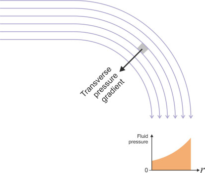
Intuitively, one understands that when the fluid changes speed there must be a pressure difference that is pushing it forward or holding it back: in other words, a pressure gradient. A positive gradient means the pressure is rising in the direction of motion, which will cause the particles to slow down, whereas a negative gradient means the pressure is falling and the particles will speed up. But the pressure can change in a transverse sense too. Put yourself in the place of a particle travelling along a streamline in two-dimensional flow within a horizontal plane: there will be other particles travelling along the neighbouring streamline to your right, and yet more travelling along the neighbouring streamline to your left. As shown in figure 3, it’s quite possible that the pressure among the fluid particles on your left is higher than the pressure among those on your right, in other words, a pressure gradient acts from left to right, across the streamlines. If so, the resulting force will deflect your path to the right.
Figure 3
If the flow is a ‘potential flow’ and we know the radius of curvature, we can use Bernoulli’s equation to calculate the transverse pressure gradient. We have previously observed that in potential flow, the velocity is inversely proportional to the radius (see equation 32 in Section F1919), and if we substitute \(k / r\) for \(U\) in equation 24, where \(k\) is a constant, we get
(30)
\[\begin{equation} p + \frac{1}{2} \rho \left( \frac{k}{r} \right)^{2} + \rho gz \quad = \quad \text{constant} \end{equation}\]Assuming that the potential pressure doesn’t vary significantly across the flow field, we can ignore the third term on the left-hand side. Now differentiate both sides with respect to \(r\), and after re-arranging the result we arrive at:
(31)
\[\begin{equation} \frac{dp}{dr} \quad = \quad \frac{\rho k^{2}}{r^{3}} \end{equation}\]showing that the pressure gradient is inversely proportional to the cube of the radius. It steepens towards the centre of the curve. Now, you may be wondering how the transverse pressure gradient relates to the centripetal force. Common sense suggests that it supplies exactly the force needed to hold each particle on its curved path of radius \(r\).
Figure 4
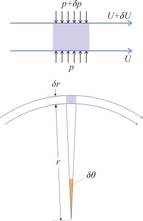
figure 4 shows a particle of mass \(m\) embedded in a fluid annulus between concentric circles of radius \(r\) and radius \(r + \delta r\). The particle subtends an angle of \(\delta \theta\) at the centre. Both \(\delta r\) and \(\delta \theta\) are infinitesimally small so the perimeter is represented as a rectangle. The flow field has a thickness of one unit. The volume of the particle is \(\delta r\) times \(r \delta \theta\) times 1, which comes to \(r \delta r \delta \theta\). Hence its mass is \(\rho r \delta r \delta \theta\), and the centripetal force acting radially on the particle must be
(32)
\[\begin{equation} \text{Centripetal force required} \quad = \quad - \frac{mU^{2}}{r} \quad = \quad -\rho U^{2} \delta r \delta \theta \end{equation}\]It has a negative sign because it acts radially inwards, in the opposite direction to the direction of increasing \(r\). After substituting \(k / r\) for \(U\), this becomes
(33)
\[\begin{equation} \text{Centripetal force required} \quad = \quad - \frac{\rho k^{2} \delta r \delta \theta }{r^{2}} \end{equation}\]Now for the force supplied by the pressure gradient. It has two components. The force acting on the outer face AB of the particle is - \(\left( p + \delta p \right) r \delta \theta\), while the force acting on the inner face CD is \(+ pr \delta \theta\). The net force on the particle supplied by the pressure gradient is the sum of these two, so that
(34)
\[\begin{equation} \text{Radial force supplied} \quad = \quad -r\delta \theta \delta p \end{equation}\]and from equation 27 we see that
(35)
\[\begin{equation} \delta p \quad = \quad \frac{\rho k^{2}}{r^{3}} \delta r \end{equation}\]so that after substituting the right-hand side for \(\delta p\) in equation 30 we finally obtain
(36)
\[\begin{equation} \text{Radial force supplied} \quad = \quad - \frac{\rho k^{2} \delta r \delta \theta }{r^{2}} \end{equation}\]which is identical to the right-hand side of equation 29. This confirms our guess that it’s the transverse pressure gradient that supplies the required centripetal force and keeps the particle on track. It is not surprising – if it didn’t there would be something amiss – but it provides independent support for the idea that when a fluid moves along a curve, the particle speed is inversely proportional to the radius. In the previous Section, we arrived at this conclusion using a purely geometrical argument; it’s a characteristic of rotationless flow that the particles towards the centre move faster than those on the outside, and very much faster close to the centre. Now we see it justified from a dynamical point of view: the inverse relationship between \(p\) and \(r\) is essential to balance the internal forces within the fluid. Later in Section F1818 the same model will reappear when we analyse the fluid motion in a vortex.
Using the equation
In principle, the Bernoulli equation lets us determine the fluid forces acting at any point on the surface of a moving body in two steps. First, we work out the fluid velocity as described previously in Section F1919, then substitute the resulting value in the Bernoulli equation to determine the pressure. In reality, the process not as straightforward as it might appear, but at least we can make a start. So let’s look at the conditions under which the method works, and go on to illustrate the procedure with an example.
When it can be applied
Our derivation of Bernoulli’s equation assumes an ideal fluid – non-viscous and incompressible - in steady, irrotational flow. Then the constant on the right-hand side has the same value everywhere in the flow field, and as we’ll demonstrate later, given the fluid velocity, equation 24 will enable us to work out the pressure at any point. In practice, no fluid meets all the conditions we’ve laid down, so among other things the value of the constant may be different for different streamlines, and while the equation will predict the pressure variations along a given streamline, without further information we can’t determine the way pressure changes across them. This may not matter for fluids of modest viscosity such as air and water because the flow tends to be almost irrotational over large parts of the flow field, and useful results can be obtained even if the fluid is not entirely friction-free. But as we’ll see in the next Section (F1917), fluid particles will rotate in areas of intense shear of the sort that occur when flowing over the surface of a moving vehicle. Particles stick to the surface and are brought to a halt. Viscous friction causes nearby particles to form a boundary layer that moves sluggishly compared to more remote parts of the fluid stream. The shear is particularly intense downstream from any sharp corner near the rear, where the boundary layer tends to ‘separate’ abruptly from the roof and sides to leave a wake. Inside the wake, the fluid motions may be erratic and the pressures lower than the Bernoulli formula predicts [5]. And there are other situations where the Bernoulli equation doesn’t apply, for example in a system where the fluid exchanges heat with its surroundings. A useful list of these cases appears in [8].
Estimating fluid pressures
For the time being we’ll ignore the boundary layer and assume ‘potential flow’. To use the Bernoulli equation, we don’t need to know the value of the constant on the right-hand side of equation 24. Instead, we can exploit the fact that it has the same value everywhere and re-cast the equation in a slightly different form: it will become a relationship linking the speed and pressure at any two points in the flow field. Label the two points 0 and 1. We can then put:
(37)
\[\begin{equation} p_{1} + \frac{1}{2}\rho U_{1}^{2} + \rho g z_{1} \quad = \quad p_{0} + \frac{1}{2}\rho U_{0}^{2} + \rho g z_{0} \end{equation}\]Now consider the point 0 to lie at a considerable distance away where the fluid motion is unaffected by any obstruction within the fluid stream. Here, the static pressure is called the undisturbed stream pressure, and we’ll denote it by \(p_{0}\). Similarly, the fluid velocity is called the undisturbed stream velocity or free stream velocity. Since in reality it is the vehicle that moves while the fluid remains stationary we’ll denote the undisturbed velocity by \(V\). On the understanding that point 0 is located at the same level \(z\) above datum as point 1 we can put \(z_{1} = z_0\), in which case the third term on the left-hand side and the third term on the right-hand side cancel out. Equation 33 then becomes
(38)
\[\begin{equation} p + \frac{1}{2}\rho U^{2} \quad = \quad p_{0} + \frac{1}{2} \rho V^{2} \end{equation}\]Notice that we have dropped the subscripts attached to the local pressure \(p\) and the local velocity \(U\) because we don’t need them any more. Equation 34 can now be arranged in the form
(39)
\[\begin{equation} p - p_{0} \quad = \quad \frac{1}{2} \rho \left( V^{2} - U^{2} \right) \end{equation}\]The quantity \(p - p_{0}\) on the left-hand side is the local pressure relative to the free stream pressure. In effect, it measures variations in the static pressure above and below the ‘ambient’ value, which for a vehicle in the open air is just the atmospheric pressure as measured by a barometer less ½\(\rho V^{2}\). If we know the local fluid velocity, we can use equation 35 to explore the pressure variations throughout the flow field provided that the fluid behaves as an ideal fluid. In particular, we can (a) work out the pressures acting on the surface of a moving vehicle, and (b) determine the pressures in areas remote from the body surface to give us an intuitive sense of how the influence of the vehicle extends out into the flow field.
Figure 5
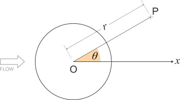
Let’s take a simple example: a circular cylinder arranged at right-angles to the flow. First, we have to determine a formula for the local velocity \(U\) at any given point P, whose position we’ll express in polar coordinates \(r\) and \(\theta\), where \(r\) is the radial distance of the point P from the origin O on the cylinder axis and \(\theta\) is the angle subtended at O, measured anti-clockwise from the \(x\)-axis as shown in figure 5. Then the velocity \(U\) can be broken down into two components, a radial component \(U_\theta\) and a tangential component \(U_{r}\). There are well-known formulae for \(U_\theta\) and \(U_r\) (see, for example [1]) and from these we can easily work out an expression for the resultant \(U\). We’ll just quote the result:
(40)
\[\begin{equation} U^{2} \quad = \quad V^{2} \left[ 1 - \frac{2a^{2}}{r^{2}} \cos 2 \theta + \frac{a^{4}}{r^{4}} \right] \end{equation}\]where \(a\) is the cylinder radius. We now substitute the right-hand side in equation 35 to get an expression for the pressure at P:
(41)
\[\begin{equation} p-p_{0} \quad = \quad \frac{1}{2} \rho V^{2} \left( \frac{2a^{2}}{r^{2}} \cos 2\theta -\frac{a^{4}}{r^{4}} \right) \end{equation}\]which can be transformed into an expression for the dimensionless ‘pressure’ \(\beta = \left( p - p_{0} \right)\)/(½\(\rho V^{2})\) thus:
(42)
\[\begin{equation} \beta \quad = \quad \frac{a^{2}}{r^{2}} \left( 2 \cos 2\theta -\frac{a^{2}}{r^{2}} \right) \end{equation}\]Figure 6
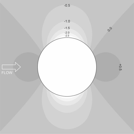
Contour lines showing how the dimensionless pressure varies over the flow field are shown in figure 6 for values of \(\beta\) ranging from -2.5 to +0.5 at intervals of 0.5. The darker shades represent areas of high pressure, while the lighter ones represent low pressure. In figure 6 we see two high-pressure zones, one upstream and one downstream of the cylinder surface. There are also two low-pressure zones, one on either side of the cylinder relative to the direction of flow; they extend over a much larger area than the high-pressure zones and the pressure variations are more intense. The contours labelled ‘\(\beta = 0\)’ mark the boundary between the high-pressure zones and the low-pressure ones: along these contours, the fluid pressure is equal to the free stream pressure. It is not difficult to show that for large \(r\), these contours approach four straight-line asymptotes arranged in the form of a cross whose arms are aligned at \(45^{\circ}\) and \(135^{\circ}\) to the \(x\)-axis and divide the flow field into four equal sectors.
Surface pressures on a moving body
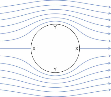
The pressure contours revealed in figure 6 are interesting, but engineers are even more interested in the pressures that act directly on the surface of a moving vehicle. Let’s continue with the circular cylinder as an example. Imagine a cargo ship with a cylindrical funnel of diameter 3 m mounted vertically on its superstructure. Its cross-section appears in figure 7. The funnel is exposed to a horizontal air stream with a relative velocity of 20 m s\(^{-1}\) (equivalent to a force 8 gale on the Beaufort scale), and given that any interference to the air flow from any other part of the ship can be neglected, we want to estimate the maximum air pressure and the minimum air pressure acting on the funnel surface.
Figure 7
We start by obtaining the fluid velocity on the funnel surface as a function of \(\theta\) by putting \(r = a\) in equation 36 to get
(43)
\[\begin{equation} U_{\text{surface}}^{2} \quad = \quad 2V^{2} \left( 1 - \cos 2\theta \right) \end{equation}\]There are two points where the pressure reaches a maximum. They occur at the two stagnation points \(\theta = 0\) and \(\theta = 2\pi\) marked with an ‘X’ in figure 7, where \(U_{surface}\) falls to zero. Now return to equation 35. By putting \(U\) equal to zero, \(V\) equal to 20 m s\(^{-1}\), and the density of air \(\rho\) equal to 1.226 kg m\(^{-3}\), we find that the pressure relative to the free stream pressure \(p - p_{0}\) is about 240 N m\(^{-2}\), representing a pressure rise of roughly 0.0024 atmospheres.
What about the minimum pressure? From equation 39 we see that the velocity peaks at the two points \(\theta = \pi /2\) and \(\theta = 3 \pi /2\) on either side of the funnel, marked by the letter ‘Y’ in figure 7. Here, the local air velocity \(U_{surface}\) comes to \(2V\), so we can put \(U\) = 40 m s\(^{-1}\) in equation 35, and with the values of\(\rho\) and \(V\) as before, we estimate the minimum pressure relative to the undisturbed stream pressure as roughly -730 N m\(^{-2}\), a drop of roughly 0.0073 atmospheres.
However, it would be unusual for a transport vehicle designer to apply the Bernoulli equation in this way. Together with the potential flow model, Bernoulli’s equation gives plausible results only for streamlined body shapes whose flow patterns closely approximate those associated with inviscid and irrotational flow. The problem with the circular cylinder is that in a viscous fluid, the flow pattern departs considerably from the one shown in figure 7 aft of its widest cross-section, and there may be no recognisable stagnation point on the downstream surface. In reality, most transport vehicles have quite complicated shapes, and even though streamlined to some degree, they generate even more complicated flow patterns. Hence their hydrodynamic behaviour is usually investigated using a combination of model testing and computer simulation. This doesn’t mean that we can dismiss the Bernoulli equation as irrelevant, because apart from anything else it underpins much of the theory that analysts need in order to carry out model testing and simulation. And in a more general sense, it throws light on several fluid phenomena that would otherwise be difficult to predict or explain even in a qualitative way.
Implications for moving vehicles
Strictly speaking, Bernoulli’s equation applies only to an ideal fluid in potential flow. However, it can provide useful information about fluid forces in more realistic situations. By way of introduction to the more rigorous treatment that follows, we’ll examine three of them now.
Scaling of fluid forces with vehicle speed
Engineers like to know how the fluid forces change when a vehicle speeds up or slows down; in particular, whether they rise and fall in direct proportion to speed, or to some other function of speed. Equation 35 points to a general conclusion. As explained in Section F1919, for an ideal fluid in steady, irrotational motion, when the vehicle velocity changes, the fluid velocity everywhere in the flow field changes in direct proportion. So, on the right hand side of equation 35, the local velocity \(U_{1}\) can be written as a constant times \(V\), and consequently the right hand side as a whole is proportional to \(V^2\). Hence when a vehicle is immersed in a potential flow, the pressure anywhere on the body surface relative to free stream pressure is proportional to the square of the vehicle speed. As we’ll see in later Sections, the situation changes in viscous flow, but not radically, and to a rough approximation, the relationship still applies. This means that the forces acting on the vehicle will grow rapidly with increasing speed.
Stagnation points
The designer is also interested in the way pressure varies from place to place over the body surface. Particularly interesting are locations where the fluid velocity falls to zero: they are called stagnation points. We’ve met stagnation points already in connection with a ship’s funnel, but they occur with almost any moving body, and there may be several dotted around a more complicated profile such as a saloon car. The dynamic pressure at a stagnation point is zero, and since it can’t get any lower, at this point the static pressure will be at its maximum possible value [2]. For simplicity let’s assume a two-dimensional flow field. As shown in figure 8, a stagnation point typically occurs at the nose where the flow divides (and also, in theory, at the tail where the flow converges again). It also occurs in places where the body surface follows a sharply re-entrant curve, notably at the scuttle [3]. These are good places to install an inlet duct, because the fluid velocity \(U_{1}\) is zero, the dynamic pressure falls to zero, and the static pressure \(p_{1}\) rises to a maximum known as the stagnation pressure whose value is equal to the total pressure \(p_{0} +\)½\(\rho V^{2}\) in the undisturbed stream.
Figure 8
A stagnation point is also a good place to install a Pitôt tube. A Pitôt tube is a device for measuring a vehicle’s speed by probing the surrounding flow field. It’s most commonly used on aircraft: in its most basic form it consists of an open-ended tube that projects through the boundary layer into the surrounding fluid. The nozzle faces upstream and causes the fluid to halt, thereby forcing a stagnation point at which the dynamic pressure falls to zero and the total pressure equals the static pressure \(p_1\), which is measured by a pressure transducer inside. A second opening on the side of the tube measures the static pressure \(p_0\) within the undisturbed stream. The difference between the two measurements gives you the dynamic pressure, and by putting \(U_{1}\) equal to zero in equation 35, after rearrangement this leads to an expression for the undisturbed stream velocity \(V\):
(44)
\[\begin{equation} V \quad = \quad \sqrt {\frac{ 2 \left( p_{0} - p_{1} \right)}{\rho }} \end{equation}\]Stability
If you are designing a vehicle you’ll be concerned about the pressure of the air or water moving over its outer shell, which can affect the way it moves. Imagine the vehicle is travelling at cruising speed and fix attention on a particular square centimetre of the body surface. You would expect the fluid forces acting on that square centimetre to have (a) a longitudinal component, and (b) a transverse component at right-angles to the direction of motion. For the moment we’ll focus on the transverse component, which could act in a lateral direction, or in a vertical direction, or in a combination of the two. Lateral forces can be dangerous, but for reasons that we’ll explain shortly we can’t use Bernoulli’s equation to predict them, and in any case, most vehicles are symmetrical about their centreline in plan and the lateral forces cancel out.
However, an exception occurs when two vehicles are moving along side-by-side, in which case their two flow patterns interact. For example, when water flows between sides of two ships sailing abreast, it accelerates through the gap, and Bernoulli’s equation tells us that the pressure will fall. The two ships are inevitably drawn together in such a way that skilled helmsmanship is needed to keep them apart. A more complicated sequence of lateral forces occurs when one ship passes or overtakes another, and a similar interaction occurs between trucks moving along a motorway.
Vertical forces can affect a vehicle’s motion too. In the case of an airship or submarine, the pressure distribution is more-or-less symmetrical about a horizontal plane through the vehicle’s longitudinal axis so again the forces cancel each other out. (For heavier-than air machines of course, there is a resultant upward force – ‘lift’ – that is vital in order to keep the aircraft in the sky, but again Bernoulli’s equation can’t account for it and we’ll deal with it separately in Section F1817, Section F1816 and elsewhere.)
Figure 9
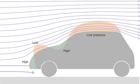
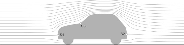
Land vehicles are different. Surprisingly perhaps, they can create ‘lift’, and this time, Bernoulli’s equation helps to explain why. We have seen that in general, streamlines crowd together as the fluid passes over a convex body. When an automobile moves along a road, the streamlines squeeze over the vehicle and around either side, with comparatively little passing underneath. The flow pattern around the front of the vehicle is shown in figure 9. Since the streamlines are widely spaced at the nose, the velocity is low and the pressure high. Then the direction of curvature reverses as they sweep over the hood (bonnet) and finally the roof. At this point they are closer together, so the velocity rises and the pressure falls. In strictly potential flow, the upward force would be balanced by a downward force acting on the vehicle floor, but in reality, friction with the road surface throttles the under-body flow, leaving a non-zero resultant force that tries to lift the car off the road, an alarming tendency that we’ll consider further in Section C1416.
So far we haven’t mentioned longitudinal forces. They are important for a different reason: they tend to slow the vehicle down. But here, as with the other cases mentioned above, Bernoulli’s equation doesn’t help. We have run into a fundamental limitation of the potential flow model, because it doesn’t take into account the viscous nature of real fluids and can’t predict some rather important aspects of their behaviour.
D’Alembert’s paradox
About 250 years ago, a brilliant French scientist tried to work out the fluid pressures on a moving body, using a method that was a direct ancestor of the one developed by Euler and his followers, the one that we have been using here. Over period of more than 20 years, Jean le Rond d’Alembert struggled with elementary body shapes, and found to his surprise that in each case the pressures acting on the body surface cancelled one another out. Consider, for example, the cylinder immersed in a uniform flow field as shown earlier in figure 6. The flow pattern downstream is a mirror image of the flow pattern upstream, and the distribution of pressure on the front and rear faces of the cylinder is exactly the same. Worse, he discovered that for a body of any shape in steady translational motion through an irrotational, ideal fluid of infinite extent, the fluid pressure could generate a couple, but there was no net force in any direction. A proof in modern notation is set out in [7]. D’Alembert had made fundamental contributions to mechanical science but couldn’t explain where resistance forces came from, or how a bird could fly.
So how does this square with what is happening to the automobile in figure 9? Owing to the low pressure zone over the roof, we know there is a net force tending to lift the vehicle off the road, whereas the potential flow model would appear to forbid it. In this case, however, the model works, because the car is not fully ‘immersed’. With the floor pan close to the ground, relatively little air gets underneath so that effectively, we are looking at only half a flow field. This becomes clearer if you return to figure 6 and imagine the cylinder together with the whole of the surrounding flow field split into two along the x-axis. Now remove the lower half, and you have a semi-cylinder with only the upper body surface exposed to the fluid, hence a net ‘lift’. As we saw earlier, the fluid forces increase as the square of vehicle velocity. If you drive almost any vehicle fast enough, it will take off.
The next step...
To his great frustration, d’Alembert never discovered the answer to the riddle. We now know that fluids have viscosity, and that viscosity leads to both lift and drag. How to deal with these viscous forces will emerge step by step as we work through different aspects of fluid flow in the Sections that follow.