© Susanna Rossini
M.1820
Ocean waves
Occasionally, the sea is calm, calm enough for you to see stars reflected in the surface at night. But that’s rare. Usually, it is scoured by the wind, forming ripples that absorb the wind’s energy and carry it with them at a leisurely pace along the water surface. Over time, the ripples join forces and grow into waves that are sufficiently powerful to break over a ship’s deck and make it roll disconcertingly from side to side. For well over a hundred years, scientists have been trying to understand their behaviour, so that meteorologists can forecast their arrival in advance and shipwrights can build vessels strong enough to withstand their impact. In this Section we’ll examine how waves are created, and how they can move over long distances before they fade away or break on a distant shore.
Figure 1
The shape of waves
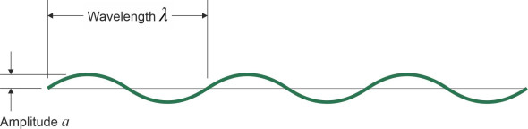
To create a mathematical model of the ocean surface, it helps to start with small waves and work upwards. By ‘small’ we mean waves of relatively small height in relation to their wavelength, which can be a long as you like. Under these circumstances, one can demonstrate from first principles that the profile of the water surface will follow a sine curve as shown in figure 1.
Figure 2
The sinusoidal profile
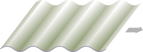
Sinusoidal waves are sometimes called Airy waves after Sir George Biddell Airy, an English mathematician who held the position of Astronomer Royal in Britain from 1835 to 1881 and made contributions to the mechanical sciences as well as optics and astronomy. Waves are a group phenomenon; rarely can a single wave exist on its own, at least not at sea. An idealised model for what happens at sea is a train of waves, all of which have the same wavelength \(\lambda\) and amplitude \(A\). Their crest are straight, arranged in parallel at equal intervals as shown in figure 2. They are known as plane progressive waves. As long as the water is fairly deep, their phase velocity \(V\) and wavelength are related by a formula that we’ll use quite often in this web site:
(1)
\[\begin{equation} V \quad = \quad \sqrt{\frac{g \lambda}{2 \pi} } \end{equation}\]The derivation is set out in the standard textbooks, for example [10]. It’s rather involved, and we won’t repeat it here. But the formula is rather important in what follows. Apart from anything else, it tells us that not all waves travel at the same speed, and in particular, that long waves travel faster than short ones. A wave of length 100 mm that fits in your kitchen sink will crawl along at 1.4 km/h, while a wave of length 200 m travels at over 60 km/h – faster than most ships.
Since all the waves in figure 2 have the same wavelength, they all travel at the same speed, so the shape of the water surface (a) looks the same everywhere and (b) apart from moving along with velocity \(V\), remains unchanged over time. Of course, a real sea is more complicated because it will usually display a mixture of waves of different wavelengths travelling in different directions. But provided each component has sufficiently small amplitude, its surface will follow a sine curve, and wherever it meets another wave component the two are superimposed - the water surface profile will trace out the sum of the individual sine curves. You can add them together, and in this sense the waves are said to be linear. However, unless they have identical wavelengths they will travel at different speeds and the water surface will evolve over time.
Figure 3
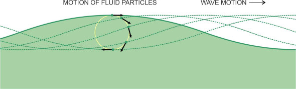
Figure 4
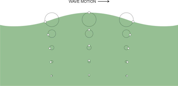
When we refer to wave motion, we are talking about the surface geometry, not the water particles themselves. For linear waves in deep water, the particles move in circles. Close to the surface, the circles are quite large, their radius \(r_0\) being equal in fact to the amplitude of the wave as shown in figure 3. But it diminishes quickly with depth, and at any given depth \(z\), the radius \(r\) is given by:
(2)
\[\begin{equation} r \quad = \quad r_{0} e^{-2 \pi z / \lambda } \end{equation}\]You can see from figure 4 that the circles are barely noticeable at depths greater than half the wavelength [4] [11].
There’s another way to visualise what is happening in a sinusoidal wave. In figure 5 we see a snapshot of the particles at a particular moment of time. They are represented by black dots, while the short line attached to each dot represents the particle’s speed and direction of motion. They don’t move very fast - their velocity is much less than the phase velocity of the waves, which is represented by the larger green arrow at the top, which in this case is moving about five times faster than the particles on the water surface.
Figure 5
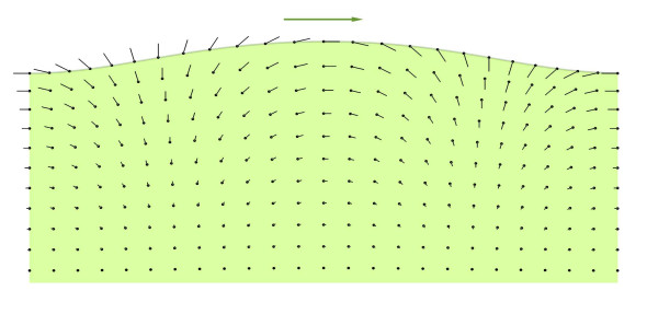
Figure 6
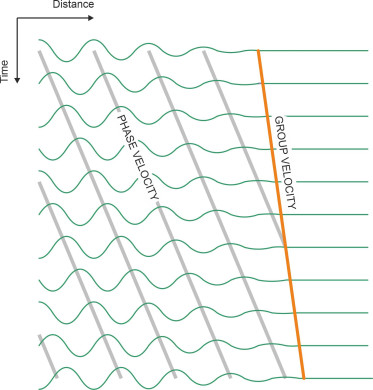
Another puzzling aspect of wave behaviour is the way they carry energy. Imagine if you will a narrow channel containing still water. If a disturbance is created suddenly at one end, a group of waves will move along the channel away from the disturbance. Assuming the individual peaks and troughs follow a sinusoidal profile, their phase velocity and wavelength will follow the relationship specified in equation 1. But considered as a group or a wave packet their behaviour is not quite as you might expect. The packet as a whole doesn’t move at the same speed \(V\) as the individual crests and troughs, in fact its speed is half that value: \(V/2\). This implies that individual waves appear almost magically at the trailing edge, travel forward until they overtake the leading edge, then vanish [2] [13]. We have tried to picture the process in figure 6, in which the wavy line across the top represents the wave packet at a particular moment of time - not the whole wave packet, just the leading edge. The lines beneath show how it evolves over time as it moves from left to right along the channel. What’s important is that the energy moves at the same speed \(V/2\) as the packet and not the individual waves.
Non-linear waves
The sinusoidal model works only for gentle waves. It is distinguished among other things by its symmetry: each trough has the same shape as a crest in the sense that the one is a mirror image of the other. But when conditions become more severe, the symmetry is lost. The crests become sharper and rise to a higher level, while the troughs become shallower and longer [3]. Such waves are non-linear in the sense that you can’t add their heights together: when two non-linear waves meet or cross one another, the total height is not equal to the sum of the individual heights. Although steeper than a sinusoidal wave, there is a limit to the slope of the surface on either side of the crest. The most steeply pointed crest has a slope equal to 30 degrees, and the height from crest to trough is limited to one-seventh of its wavelength or \(0.14 \lambda\) [12] (figure 7). Anything higher is unstable: as the wave grows in height, the circular orbits of particles in the crest increase in diameter and the particles themselves must orbit at higher and higher speed. When the velocity of particles at the tip of the peak becomes greater than the phase velocity of the wave itself, the top ‘falls over’ – in other words, the wave breaks. This can happen under rough conditions in open water, where under very high and sustained wind speeds, most waves will break, which is potentially dangerous for smaller boats [1].
Figure 7
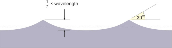
Figure 8
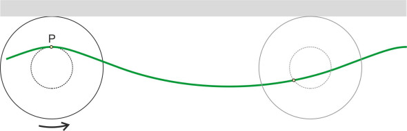
The trochoidal profile
In contrast with the linear case, there is no simple model for non-linear waves. A good model should (a) satisfy the underlying equations of motion (which we haven’t gone into here) and (b) allow the waves to retain their shape in a stable fashion as they propagate across the ocean surface. The trochoidal curve is a compromise, and in spite of its theoretical shortcomings [12] it is widely used in ship design. Like a sinusoidal wave it assumes that the water particles are moving in circular orbits, and one can use it to simulate realistic-looking waves with profiles ranging from the sinusoidal to a sharply-crested peak, simply by changing the model parameters. The trochoid is the curve traced out by a point on a rolling disk – we came across the special case where the point is marked on the tread of a railway wheel in Figure 12 of Section R1604. To generate a water wave, we must turn the picture upside down and imagine a horizontal rail mounted above the water surface, with a wheel of radius \(R\) pressed up against the surface and rolling along underneath as shown in figure 8. Now mark a point P on the disk vertically above the disk centre at radius \(r\) and rotate the wheel anticlockwise. The point P will move downwards and to the right. If we denote the horizontal distance by \(x\), and the vertical distance by \(z\) (measured positive downwards), then the curve that P traces out is described by the two simultaneous equations:
(3)
\[\begin{equation} x \quad = R \theta - r \sin \theta \end{equation}\](4)
\[\begin{equation} z \quad = r \left( 1-\cos \theta \right) \end{equation}\]where \(\theta\) is the angle through the wheel rotates anti-clockwise from its starting position. In one revolution, the disc moves forward a whole wavelength \(\lambda\), and since its circumference is \(2 \pi R\), the radius \(R\) must be equal to \(\lambda / 2 \pi\). The curve shown in figure 8 has a wavelength of 10 m and derives from a disc of diameter \(10/2 \pi = 1.592\ \text{m}\). It was traced out by a point located on the disc at a radius of \(40 \%\) of the overall diameter, equal to 0.637 m. The wave height from crest to trough is \(2 \times 0.637 = 1.274\) m. More curves generated with the same disk are shown in figure 9, each arising from a different value of the parameter \(r\).
Figure 9
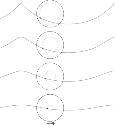
Figure 10
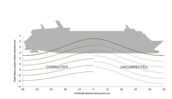
Because it can represent waves of different ‘peakiness’, the trochoidal model was adopted many years ago by designers for estimating the impact of waves on a hull. Waves can arrive from any direction, and the designer tries to judge which of them pose a significant threat. Here we’ll focus on the case where a wave approaches from ahead or astern, passing underneath the hull until it is supporting the ship at its centre as shown in figure 10. Given a trochoidal wave surface, what can we say about the water pressure acting on the plating around the submerged part of the hull? This is a complicated matter because the neither the water particles nor the ship are stationary – in fact they are both undergoing acceleration with the rise and fall of the water surface. The problem is dynamic. But by comparison with the forces acting on the suspension of an automobile, they vary quite slowly. As a first approximation, engineers used to treat the problem as static, as if the ship were poised on the crest of a wave frozen in time. This simplified the analysis because they could equate the pressure acting at any point on the hull surface to the depth times the density of seawater. Carried out over the whole of the submerged area of the hull, this enabled them to plot contour lines of equal pressure whose wavy profile echoed the surface profile of the wave.
The pressure contours of a wave that is 6 m high and 100 m long are shown in figure 10. The diagram is split into two halves. On the right-hand side we see the contours plotted as if the pressure increased uniformly with depth, as it does in still water. However, the motions of the water particles diminish with depth: as we saw earlier, for a sinusoidal wave the orbit radius varies according to equation 2, and below a certain depth it becomes negligible. In the case of a trochoidal wave, the orbit radius satisfies [17]:
(5)
\[\begin{equation} r \quad = \quad r_{0} e^{-z/R} \end{equation}\]Assuming the pressure variations diminish in the same way, one can plot a ‘corrected’ version of the static pressure contours, and these are the contours that appear on the left-hand side of figure 10, where the vertical scale is exaggerated in order to bring out the differences. You can just see that the pressure acting on the bottom of the ship’s hull is reduced in the region of the wave crest, as if the fluid were somehow less dense than ordinary seawater. By contrast, the pressure in the troughs is increased, as if the fluid were more dense than seawater. The combined effect is to spread the load over a greater length of hull, which would ease the stress in the plating.
Adjustments of this kind have routinely been applied by designers for over a hundred years, in connection not only with heaving and pitching motions but rolling motions as well, where the adjustment can make an appreciable difference to the estimate of the righting lever [15]. The process is known as ‘Smith’s correction’, and you can find some of the details in [16]. But not all wave pressures can be treated in this way because some involve dynamic impacts, for example when the bottom of the ship ‘slams’ onto the water surface as the bow plunges into a deep trough. We’ll return to this topic later in Section M1115.
The wave climate
To understand wave conditions at sea, it helps to break down the problem into three parts: (a) how waves begin, (b) the pattern of waves at any particular location – the wave climate, and (c) individual, extreme waves often called rogue waves.
Wave development
We saw earlier in Section M1919 how the wind triggers the formation of ripples on the water surface. The next question is how they grow into waves of significant size. Experience has shown that there are three important factors: the fetch (the uninterrupted distance that the wind blows across the surface), the strength of the wind, and its duration. To see how they interact, we’ll picture how the waves change over a large, uninterrupted body of water. We are standing at the shoreline facing the sea, and the wind is blowing from behind us onto the water at a steady velocity \(V\). Nothing much is happening at the shoreline, but further out, waves appear whose intensity increases with distance from the shore. There are five main stages in the development process: ripple, chop, sea, swell and decay.
- As it leaves the near shore, the wind stirs up ripples on the water surface.
- In turn, the ripples give the wind a better ‘grip’ on the surface. Further offshore, the wind is blowing over a longer fetch, and the water becomes choppy. At this stage, the waves have grown in height and wavelength, and according to equation 1, must be travelling more quickly than they were close to the shoreline. But they’re not yet travelling as fast as the wind itself.
- The waves continue to gather energy from the wind, growing in size and accelerating steadily as they do so. It used to be thought that as they approached the same speed \(V\) as the wind, they would stop growing: the waves would be ‘fully developed’. But we now know that the waves exchange energy among themselves.
- The larger waves absorb energy from the weaker ones and then leave them behind as they continue to grow in height, wavelength and speed. This means they can out-run the wind.
- The waves form ‘whitecaps’ that break in open water, dissipating energy through friction and turbulence. Eventually, they will reach an area where the wind is less severe, and die out (a) by fanning out over a wider area, or (b) by breaking on a distant shore.
The first four stages assume a particular value of the wind speed \(V\). But what happens if we re-run the process with the wind blowing harder, for example, at double the speed? The wave height throughout will increase in proportion to \(V^2\) [14], so that the waves will reach any given height in a shorter fetch, and their maximum height will increase by a factor of 4. Notice that the water particles inside a wave crest don’t actually go anywhere – only the energy is propagated, and since the fluid motions themselves are relatively small, the friction losses are small. Hence waves can travel for a considerable distance after they have formed without further help from the wind. During the course of his research, the celebrated oceanographer Walter Munk once detected waves that had travelled from Antarctica to Alaska, a distance of 7000 miles.
Wave height
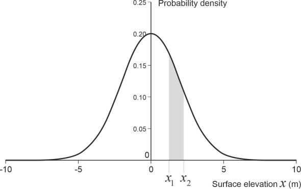
Up to now, we have pictured waves arranged in orderly ranks like soldiers on parade. However, this is not what actually happens. Out in the open sea, waves tend to arrive in a chaotic jumble: ‘short-crested waves’ that vary in amplitude, frequency and direction. This is because they are a mixture, having arrived from different directions and often from different sources. Figure 11 shows a pattern synthesised by the author from just three plane progressive waves and plotted on a spreadsheet. Each of the three components has a different wavelength, amplitude, and direction of travel, all specified by a random number generator. In a real situation at sea, there could be (a) a swell left over from a storm the previous day, (b) the same swell arriving via a different route have been refracted around some coastal feature, and (c) waves created locally by the current breeze. The result is a wave ‘climate’. This raises two problems: how to quantify the mixture in simple terms, and how to predict the wave climate given the wind velocity over a given time period. This is essentially a problem in statistics. We’ll start by looking not at the waves as such, but the elevation \(x\) of the water surface measured relative to the mean water level. At any given moment at any given location, the elevation \(x\) will be the outcome of many random processes. Then according to the Central Limit Theorem, the value of \(x\) will tend to follow a Gaussian distribution [6], whose probability density function (p.d.f) is the familiar bell-shaped curve shown in figure 12. The curve shown relates to a sea with a root mean square surface elevation of 2 m. If you choose any two values \(x_1\) and \(x_2\) on the horizontal axis, the area under the curve between those two values tells you the probability that the water surface level lies between them at any given moment. Since the water level frequently passes through zero, the summit of the curve is centred at \(x = 0\).
Figure 11
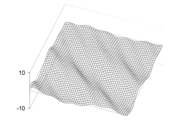
Figure 12
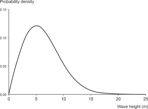
Of course, ship designers really want to know about the crests as opposed to the level of the water surface in between. Since we are looking at a jumble of waves superposed on one another, the crests themselves will vary randomly in height from one wave to the next. If we denote the elevation of a wave crest by \(x_c\), then on the assumption of Gaussian elevations and a narrow frequency bandwidth, it can be shown that the p.d.f. of \(x_c\) follows a Rayleigh distribution thus:
(6)
\[\begin{equation} f(x_c) \quad = \quad \frac{x_c}{m_0} e^{-{x_c}^2 / 2 m_0} \end{equation}\]where \(m_0\) is a fixed parameter equal to the mean square of the wave crest heights. The shape of the p.d.f. is illustrated in figure 13 for the particular case where the mean square wave elevation \(m_0\) is \(25 \text{ m}^2\). The curve has a fixed shape, but it can be re-scaled horizontally for different values of \(m_0\) (provided it is re-scaled vertically too, so that the total area under the curve remains equal to one). Notice that it is not symmetrical, having a long upper ‘tail’. The tail represents the highest waves, the ones that are most likely to damage a ship.
Figure 13
For convenience, oceanographers have conceived a simpler measure called the significant wave height, defined as the average height of the highest one third of waves. It enables one to make quantitative comparisons between sea conditions in different places in terms of a single number. Until it was adopted by regulatory authorities, mariners had to rely on a subjective scale, a set of ‘sea state codes’ - verbal descriptions devised in the 1920s by Captain H P Douglas for the British Navy [9]. Later, the World Meterological Organisation designated specific values of the significant wave height corresponding to each division of the Douglas scale as shown in table 1 [22].
| Code | Description of sea state | Significant wave height (m) |
|---|---|---|
| 0 | Calm (glassy) | 0 |
| 1 | Calm (rippled) | 0.00 - 0.10 |
| 2 | Smooth (wavelets) | 0.10 - 0.50 |
| 3 | Slight | 0.50 - 1.25 |
| 4 | Moderate | 1.25 - 2.50 |
| 5 | Rough | 2.50 - 4.00 |
| 6 | Very rough | 4 – 6 |
| 7 | High | 6 – 9 |
| 8 | Very high | 9 – 14 |
| 9 | Phenomenal | Over 14 |
Wave spectrum
Sea state codes are useful for describing the wave conditions at a particular place and time, but when designing a ship, it is important to know how often the extremes are likely to occur, so the hull can be built to withstand them. Put simply, we need a more detailed picture of what is going on. It’s not just the height of the crests that matters, but the time intervals between them. There’s a practical reason for this: ships roll from side to side, and the natural period of oscillation often lies in the region of 10 seconds [6], corresponding to a frequency of 0.1 Hz. Waves whose frequency lies close to this value can set up a resonant motion leading to extreme roll angles and a possible capsize. Ideally therefore, for any given wind speed, our model should predict both the wave height and frequency.
It was a famous mathematician who made the first steps in this direction. Norbert Weiner (1894-1964) is better known for developing the theory of signal processing that engineers still use to design control systems for machines and robots. He was inspired by gazing at the River Charles from his office at Massachusetts Institute of Technology, wondering how he could characterise the apparently random waves on the water surface. His solution was the wave spectrum. We’ve come across it before. You’ll recall that in Section C1603 we introduced a function called the power spectral density in connection with road surfaces. The idea is to visualise the bumpiness of a road surface as a superposition of sine waves and cosine waves. The waves feed into the suspension of a moving car at many different frequencies. A weak component or signal (corresponding, for example, to microscopic roughness on the surface of each gravel particle embedded in the road surface) might have an amplitude of less than 1 mm. On the other hand, potholes generate strong signals with an amplitude of several millimetres, enough to shake the suspension and make the ride uncomfortable. The totality can be pictured in the form of a power spectral density curve or PSD for short, that represents the relative strengths of the signals at different frequencies.
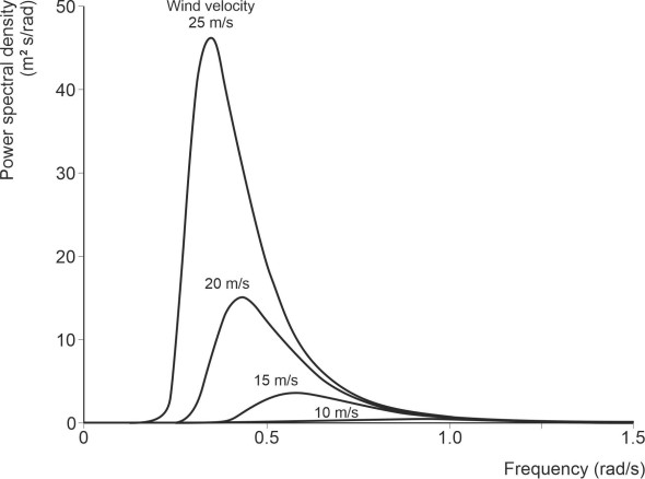
The same technique can be applied to ocean waves, where the input ‘signal’ is the instantaneous water surface level at the given location. The power spectral density curve represents its relative strength at different frequencies. Here, we’ll denote the frequency by \(f_s\), and measure the strength \(F(f_{s})\) of the signal in terms of the amplitude squared not the amplitude itself. It has units of ‘square-metres-per-(cycle-per-second)’ or equivalently m2s. The total area under the curve equals the overall mean square amplitude, while the area under the curve between any two frequencies tells you the mean square amplitude of waves lying within that bandwidth. For many years, a curve fitted to observed water surface levels was used to delineate the power spectral density curve for ocean waves as a function of wind speed. Curves for this model, the Pierson-Moskowitz model, are shown in figure 14. The curves show that as the wind speed increases, two things happen: (a) the wave heights increase, and (b) the frequency falls.
Figure 14
Since these curves first appeared, events have moved on. Research carried out as part of the JOint North Sea Wave Project (JONSWAP) has led to more sophisticated models that we won’t go into here [7]. It also revealed that waves tend to spread out, usually within \(\pm 30^{\circ}\) of the wind direction. Building on research of this kind, meteorologists and oceanographers have developed computer simulation models that can predict wave conditions across most of the world’s oceans. You can download the forecasts from the US National Weather Service web site listed at the end of this Section [21].
Waves and ships
In this Section, we’ve touched on the behaviour of ocean waves and how they can be modelled or represented, culminating in the idea of a spectrum or mixture of waves of different frequency. But to understand the effects of a heavy sea on the structure of a ship’s hull and the people on board, we’ll need to know how individual waves present themselves to the vessel in the open sea. We’ll start by thinking of the sea as a rough surface, and later in Section M1115 imagine how the hull responds to the ups and downs it encounters during a voyage. This is essentially what an automobile designer does when developing the suspension for a new model: the idea is to model the process as an input/output system. As explained in Section G1115, the input consists of irregularities in the road surface, which are ‘processed’ by the tyres, springs and dampers, to yield an output as perceived by the passengers in the form of oscillations in the seats and bodywork.
How rough is the sea?
Picture the sea frozen in time, its surface punctuated with random bumps and hollows like any patch of land onshore. We can quantify the roughness by choosing one of the Pierson-Moskowitz curves that appear in figure 14 and translating it into a slightly different form. This means plotting the spectral density as a function of wavelength rather than frequency. We’ll process just one of the curves, the one corresponding to a moderate gale with a wind speed of 15 m/s. The transformation is a fiddly process so we’ll omit the details and go straight to the result, namely the blue curve in figure 15. Both axes are plotted on a logarithmic scale. To begin with, the curve rises steadily with wavelength, showing, as one might expect, that the longer the wave, the greater the amplitude or height. But the curve peaks at a wavelength of about 200 m followed by a rapid decline. The decline reflects the fact that because it is a fluid, over very large distances the sea surface is fixed at a more-or-less constant level.
Figure 15
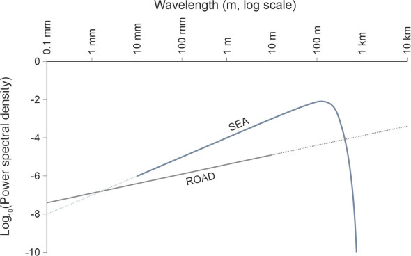
Also shown for comparison is the equivalent curve for a road surface. It represents a minor road typical of northern Europe [18]. The curve is based on data collected for a relatively short length of carriageway so one can’t be sure what it looks like for wavelengths greater than about 10 m, but it seems unlikely to peak within the range depicted because roads have ‘roughness’ on a very large scale: they go up and down hills that are many kilometres long. As you might expect, for the sea and the road that we have chosen to model here, the sea is much ‘rougher’ for wavelengths up to 500 m because of the wind-driven waves.
Interestingly, the sea is rougher than the road even at short wavelengths of the order a few millimetres as well. But if you travel on a ship you won’t notice any bumps or vibration associated with wavelengths of this order. This is because a ship’s hull processes roughness in a different way – unlike a car tyre, it simply bridges over the crests, so that waves that are less than half the length of the hull have little impact. Among other things, this means that small boats and large ships perform differently in a rough sea: a small boat will be less comfortable to ride in, bobbing up and down with every disturbance on the water surface and at risk of being swamped. But it won’t break. By comparison, a large ship won’t be much affected by short waves. On the other hand, as we’ll see in Section M1115, it may bridge across the long ones in a way that puts the structure under considerable stress.
Finally, a note on the effect of vehicle speed. The faster you drive your car, the higher the frequency of the input signal on a bumpy road. But at least the road surface is stationary so the vibration will cease when you pull over and stop. By contrast, the surface of the sea is moving all the time, and if you drop anchor, you will still be buffeted by the waves. It may be tempting to run before the wind in the hope of avoiding the waves completely, but even at full speed ahead, you will not outrun them all. A 200 m-long wave travels at over 60 km/h.
Rogue waves
Scientists are still trying to determine the largest possible size for an ocean wave. In the past, mariners occasionally reported ‘rogue waves’ over 25 metres tall [20], but since one can’t easily measure the height of a wave from a moving ship, such claims were not widely believed. However, on the basis of the data accumulating from recording instruments on buoys, oil platforms and research vessels, it seems the mariners may have been right. So how to define a ‘rogue wave’? A pragmatic definition is that it’s a wave whose height is twice the significant height of the population as a whole. As such, it will stand out from its neighbours, with a steep front and a sharp peak followed by a long trough. The first rogue wave to be measured with scientific accuracy occurred on New Year’s Day in 1995 at the Draupner North Sea oil platform. At 26 m (85 feet), it was more than twice the significant wave height, which marks it out as a statistically rare event. But there have been larger ones since. Until the year 2011, the highest ever reading was generated at a buoy off the coast of Taiwan during the typhoon Krosa in 2007. It was 32.3 m (106 ft) high [8].
Extreme waves can do serious damage. For example, in 1968 an oil tanker, the World Glory, broke in two amid severe wave conditions in the Agulhas Current. Only a few of the crew survived. It was one of many ships lost during the last century, some of which disappeared without trace, either broken or overwhelmed in remote waters. In the year 2000 an international team of scientists launched a project in order to find out what was happening. Funded by the European Union, the project was called MAXWAVE. It established that 245 of the ships lost during the period 1995-1999 had probably encountered extreme waves [20]. The researchers also studied photographic satellite images and extracted large samples of wave height. They found that the so-called ‘rogue waves’ were (a) short-lived, and (b) no more or less frequent than would be predicted by a statistical model such as the Rayleigh distribution. In other words, the data didn’t mark them out as uniquely different from the wider population.
Where they happen
But this doesn’t rule out one or more distinct physical mechanisms as a contributory factor. Research continues on possible causes that might enable rogue waves to be predicted more reliably in advance. Here are some of them:
- Waves meet on oncoming ocean current.
- A wind gust generates large waves that overtake preceding ones and momentarily gain in height when they collide.
- Two wave trains meet at an angle to form a cross-sea: when the peaks intersect, their heights are momentarily added together to create a higher one.
- Non-linear waves gain energy from other waves.
What happens when a wave train meets a current can be spectacular. We have already mentioned the Agulhas Current, the site of many losses in the past. Another example is the ‘Bermuda Triangle’, through which the Gulf Stream flows at 3 to 4 knots along a narrow channel. Covering an area of 4000 square miles between Puerto Rico, Miami, and Bermuda, the Bermuda Triangle is often stormy with very high waves. It is claimed that around 5000 people have disappeared here without trace, mostly before they could radio for help. The causes are difficult to substantiate because the Gulf Stream can drag a wrecked ship for 200 miles, leaving nothing behind for the search team to find at the scene.
An afterthought
Extreme waves can swamp a vessel, roll it over, or break it in two, but they’re not the only threat to shipping. Later in Section M1115 we’ll see that more modest waves can upset the balance of a vessel if their frequency coincides with the ship’s natural period of roll. But not all waves are bad news. Surprisingly, a tsunami is unlikely to damage a ship sailing offshore in deep water, where tsunami waves are only of the order of a metre high. In theory, such a wave can move faster than the speed of sound (many tsunamis have travelled across the ocean at not far short of supersonic speed) but the crest is spread out over a length several kilometres in the direction of motion. As perceived from the deck of a ship in its path, the slope is gradual, and such a wave could pass under the hull unnoticed.
Acknowledgement
Photo on opening page Azur by Susanna Rossini (https://susimagin.com/).