F.1518
Propeller thrust
In order to move, a vehicle must push against its surroundings. If it rests on solid ground, it will have something to push against, but if it’s floating on water or flying through the air, it can’t get a grip and must do something else. Usually, this means throwing something astern. For example, a ship uses its propeller to accelerate water, sucking it from under the hull and projecting it rearward at speed. An aircraft propeller works in the same way except that it’s usually mounted at the front rather than the rear, and it spins a lot faster. In either case, to accelerate the fluid, the propeller must apply a rearward force, and it’s the reaction to this force that causes the vehicle to move. In Section F1513, we examined the geometry of a typical propeller blade, and saw how it applied pressure to the fluid to generate thrust. Here, we’ll step back and view the wider interaction between the propeller and its surroundings. It’s interesting to see how it changes the pattern of flow in the neighbourhood of the propeller ‘disc’. Among other things, the propeller blades transfer energy into the fluid slipstream, and this energy plays no part in the vehicle’s propulsion. It is wasted: an inevitable consequence of using a fluid to generate thrust. In this Section, we’ll try to model the energy flows and ask what can be done to minimise the losses.
Axial momentum theory
Let’s begin with the scene pictured briefly in the previous Section: you are marooned in a boat in the middle of Crocodile lake. The hull is leaking, there are no oars, and the outboard motor has broken down. The question is how to reach the shore. All you can do is scoop up water from the bilges in a plastic bag and hurl the water astern, counting on the reaction to drive the boat forward. At this point, there emerges an interesting challenge. You will need to repeat the operation many times, and you don’t want to get tired too quickly. How much water should you collect for each ‘throw’, and how hard should you throw it?
Action and reaction
For your first ‘throw’, suppose you set a target speed of \(V\). Denote the mass of the boat by \(M\), and the mass of the water in the bag by \(M_{\text{water}}\). Before you throw the water, it has zero speed and therefore zero momentum. Likewise for the boat. You now hurl the water astern at velocity \(-V_{\text{water}}\) (it has a minus sign because we are measuring speeds as positive in the forward direction), so its momentum becomes \(-M_{\text{water}}V_{\text{water}}\). Ignoring the small change in the mass of the bilgewater, the momentum of the boat becomes \(MV\). There are no other forces acting on the vessel and the total momentum after the event equals the total momentum before, so we know that
(1)
\[\begin{equation} MV - M_{\text{water}}V_{\text{water}} \quad = \quad 0 \end{equation}\]which implies that
(2)
\[\begin{equation} M_{\text{water}}V_{\text{water}} \quad = \quad MV \end{equation}\]For any given target velocity \(V\) the product \(MV\) is fixed, which in turn fixes the product \(M_{\text{water}}V_{\text{water}}\). To get the result you want, you can throw a small mass of water at high speed, or alternatively a large mass of water at low speed. There’s a whole range of combinations in between that will do, as long as the product \(M_{\text{water}}V_{\text{water}}\) equals the product of the boat mass and target speed. When you accelerate the water in the bag to velocity \(-V_{\text{water}}\) you are putting kinetic energy into it. By definition, the kinetic energy is half the mass times velocity squared, hence:
(3)
\[\begin{equation} \text{Work done by you} \quad = \quad \frac{1}{2}M_{\text{water}}{V_{\text{water}}}^2 \end{equation}\]Substituting for \(M_{\text{water}}V_{\text{water}}\) via equation 2 leads to
(4)
\[\begin{equation} \text{Work done by you} \quad = \quad \frac{1}{2}\left( MV \right)V_{\text{water}} \quad = \quad \text{constant} \times V_{\text{water}} \end{equation}\]which demonstrates that irrespective of the mass of water in the bag, the energy you expend is proportional to the speed \(V_{\text{water}}\) with which you throw it. If you halve \(V_{\text{water}}\) and double the mass \(M_{\text{water}}\), you halve the energy cost. The best strategy is to throw something heavy, but not very fast.
The stream tube
One can apply the same idea to a propeller. Of course, the propeller doesn’t throw bags of water over the stern; rather, it accelerates the fluid rearwards in a steady stream. In what follows we’ll analyse the flow in terms of an idealised mathematical model that was originally devised by William John Macquorn Rankine (1820-1872) [17], a Scottish civil engineer once described as ‘the father of engineering science’ in his home country. His model was later elaborated by William Froude [11]. The idea is to ignore the pressure pulses generated by the propeller blades. Instead, the propeller becomes an actuator disc, an imaginary membrane of area \(A\) that draws fluid towards it and propels it astern. The disc is permeable, and the fluid that passes through it is enclosed within an imaginary tube - the stream tube, shown in side elevation as the blue area in figure 1. We’ll follow the progress of a chunk of fluid along the tube, through the disc, and into the slipstream, ignoring anything that happens outside. Throughout, the fluid is considered as frictionless and incompressible. The flow remains steady over time, the velocity profile is uniform at each cross-section, and the propeller blades impart no angular momentum to the fluid in the vehicle wake.
Figure 1
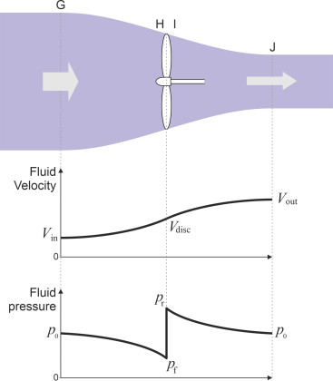
Ahead of the propeller at reference point G, the stream tube is cylindrical in shape, and the diameter of the cylinder is larger than the diameter of the propeller disc because in normal circumstances the fluid is not compressible: it speeds up as it approaches the disc, so the tube must shrink as it passes through the propeller disc, but it resumes a cylindrical shape downstream at reference point J, where the slipstream has a smaller diameter than the propeller.
Now let’s track a particle of fluid along the tube. Denote the velocity of the particles upstream at G by \(V_{\text{in}}\) relative to the propeller disc (in an ideal world this would be equal to the vehicle’s forward speed \(V\), but in the case of a ship, we replace \(V\) by the advance velocity \(V_\text{a}\), which takes into account the way the fluid upstream is entrained within the hull boundary layer). As it approaches the propeller, the fluid velocity increases, reaching a value denoted by \(V_{\text{disc}}\) at the propeller disc, through which it passes as if the disc were completely permeable. The speed continues to increase to its final value \(V_{\text{out}}\) downstream at J. But what about the fluid pressure? The pressure variation follows a different profile. Upstream at G it is equal to \(p_0\), the static pressure of the undisturbed fluid at rest. As the fluid heads towards the propeller, the pressure falls to a value \(p_{\text{f}}\) at the front face H, then rises abruptly to a value \(p_{\text{r}}\) at the rear face I. Downstream at J it decays to the static pressure \(p_{\text{0}}\) again. The fluid is driven aft by the falling pressure gradient both upstream and downstream of the disc, while the propeller is driven forward by the difference in pressure across the disc. This is the standard model for representing the action of a propeller on a fluid, albeit a simplified one [6] [18]. It applies in principle both to ship propellers and aircraft propellers [12]. So let’s derive an expression for the propeller thrust \(F\).
Thrust
During a time interval of duration \(t\), the volume of fluid passing through the disc equals the cross-sectional area \(A\) times the speed \(V_{\text{disc}}\) times \(t\). The mass \(M\) of this fluid ‘parcel’ is its volume times its density, so
(5)
\[\begin{equation} \text{Mass } M \text{ of fluid in time }t \quad = \quad \rho AV_{\text{disc}}t \end{equation}\]Overall, the speed of the fluid increases from \(V_{\text{in}}\) at G to \(V_{\text{out}}\) at J. The momentum of the fluid parcel as it passes through G is \(MV_{\text{in}}\), and its momentum as it passes through J is \(MV_{\text{out}}\), so the increase in momentum is \(MV_{\text{out}} - MV_{\text{in}}\) and the rate of change of momentum \(M(V_{\text{out}} - V_{\text{in}})/t\) per unit time. According to Newton’s Second Law, the thrust delivered by the propeller must be equal to the rate of change of momentum so that
(6)
\[\begin{equation} F \quad = \quad M\left( V_{\text{out}} - V_{\text{in}} \right)/t \end{equation}\]which after substituting for \(M\) via equation 5 leads to
(7)
\[\begin{equation} F \quad = \quad \rho AV_{\text{disc}}(V_{\text{out}} - V_{\text{in}}) \end{equation}\]To achieve any given thrust \(F\) the designer has a choice: either to make \(A\) large and the fluid velocity increment \((V_{\text{out}} - V_{\text{in}})\) small, or vice versa. In other words, one can have a large propeller turning slowly, or a small propeller turning fast, or a compromise between these two extremes. However, not all the possible combinations are equally efficient in energy terms because there is a built-in energy loss. In order to generate thrust, the propeller must inject energy into the surrounding fluid, which is carried downstream and dissipated into the ocean. The question is how the designer can manipulate the system to minimise this loss.
Saving energy
To help answer this question, the nineteenth century scientists set up a numerical indicator: the ‘ideal’ efficiency \(\eta_{\text{ideal}}\). It’s an elusive concept (at least, it puzzled me when I first became interested in the subject). You might find it helpful to divide the action of a propeller into two parallel processes. The first concerns the interaction between the blades and the surrounding fluid, which involves a transfer of energy from the engine to the water, of which a proportion – hopefully a small proportion – is lost in fluid friction and turbulence. The transfer is not 100% efficient. The second process concernes the fluid flow in the stream tube: the fluid accelerates as it passes through the propeller disc, and it’s this acceleration that determines the thrust. The ideal efficiency is concerned only with the second process, and it ignores any losses that occur at the interface between the propeller blades and the surrounding fluid. To find its value we must calculate how much energy has been expended on moving the vehicle during the time interval \(t\) (in other words, ‘useful output’) compared with the energy input from the propeller during that time. The useful output is the thrust \(F\) exerted by the propeller times the distance \(Vt\) moved by the vehicle, in other words, \(FVt\). If we assume \(V = V_{\text{in}}\) then substituting for \(F\) via equation 7 we can write
(8)
\[\begin{equation} \text{Useful output} \quad = \quad FV_{\text{in}}t \quad = \quad \rho AV_{\text{disc}}(V_{\text{out}} - V_{\text{in}}) V_{\text{in}} t \end{equation}\]On the other hand, the work supplied by the propeller equals the energy that it puts into moving the fluid. By definition, the kinetic energy of the fluid parcel at G is \(MV_{\text{in}}^{2}/2\), and its kinetic energy at J is \(MV_{\text{out}}^{2}/2\), so the work supplied by the propeller over time \(t\) is the difference between the two:
(9)
\[\begin{equation} \text{Total input} \quad = \quad \frac{1}{2}M\left({V_{\text{out}}}^{2}-{V_{\text{in}}}^{2} \right) \quad = \quad \frac{1}{2}\rho A V_{\text{disc}} \left( {V_{\text{out}}}^{2} - {V_{\text{in}}}^{2} \right)t \end{equation}\]Hence the ideal efficiency can be written
(10)
\[\begin{equation} \eta_{\text{ideal}} \quad = \quad \frac{\text{Useful output}}{\text{Total input}} \quad = \quad \frac{\rho AV_{\text{disc}}(V_{\text{out}} - V_{\text{in}}) V_{\text{in}} t}{\frac{1}{2}\rho A V_{\text{disc}} \left( {V_{\text{out}}}^{2} - V_{\text{in}}^2 \right)t} \end{equation}\]After simplification this reduces to
(11)
\[\begin{equation} \eta_{\text{ideal}} \quad = \quad \frac{2V_{\text{in}}}{V_{\text{out}} + V_{\text{in}}} \quad = \quad \frac{1}{1 + \frac{1}{2}\left( \frac{V_{\text{out}} - V_{\text{in}}}{V_{\text{in}}} \right) } \end{equation}\]And we can further simplify matters by noticing that the term \((V_{\text{out}} - V_{\text{in}} )/V_{\text{in}}\) is just the proportional change in fluid velocity as it moves through the disc. It’s conventional to define the inflow factor \(a\) as half this proportional change, in which case equation 11 becomes
(12)
\[\begin{equation} \eta_{\text{ideal}} \quad = \quad \frac{1}{1+a} \end{equation}\]This equation highlights the main disadvantage of a propeller: in order to work, it must create axial momentum in the propeller slipstream, which means that a proportion of the engine power is diverted into moving the fluid rather than into moving the vehicle. While we’re on the subject, the propeller also generates angular momentum in the slipstream because the propeller causes the fluid to rotate as it passes through. Suppose the angular velocity within the stream tube rises from zero upstream to \(a'\omega\) at the disc, where \(\omega\) is the angular velocity of the propeller disc. Assuming that the change arises independently of any change in the axial momentum, it can be shown [10] that the angular velocity downstream will be \(2{a}'\omega\) and that the ideal efficiency is accordingly reduced by an additional factor \(1-{a}'\) thus:
(13)
\[\begin{equation} \eta_{\text{ideal}} \quad = \quad \frac{1-{a}'}{1+a} \end{equation}\]So how best to summarise what is going on? For the purpose of this exercise, the input speed is fixed (we’ve assumed it is equal to the vehicle’s forward speed \(V\)). The only variable quantities are the changes that take place downstream. From equation 13 it is clear that when the changes are large, the efficiency is low. Conversely, when the changes are small, the efficiency approaches \(100\%\). The ideal efficiency is maximised when both \(a\) and \(a'\) are as close as possible to zero. Together with equation 7 this implies that in order to maintain any pre-determined level of thrust the designer should aim for the smallest possible speed drop across the propeller disc. Figure 2 shows what happens if you double the area of the propeller disc: as with the previous case of the boat propelled by hurling water overboard, it seems a good idea to move a large amount of fluid but not too fast.
Figure 2
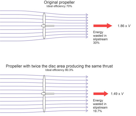
The way to do this is to have a large, slowly turning propeller. But a large propeller takes up a lot of room, and it has several other disadvantages including cost, weight, and a greater likelihood of accidental damage, so it’s useful to know what are the potential gains in relation to the costs – in particular, how much larger should the propeller be to achieve a specific pay-off? A good measure of the ‘pay-off’ is the improvement in ideal efficiency, or equivalently, the reduction in energy wasted in the propeller slipstream. Let’s take a simple example. Figure 2 depicts a propeller with an ideal efficiency of \(70\%\). The fluid velocity \(V_{\text{out}}\) in the slipstream is 1.86 times the input velocity \(V_{\text{in}}\). Can we improve the propeller’s efficiency by making it larger? Calculations show that if we double the disc area while maintaining the same thrust, the ideal efficiency increases to \(80.3\%\). Is this a worthwhile improvement? If you’re interested, you’ll find more details set out in the Appendix.
Dimensional analysis
We are treating the propeller as an ‘actuator disc’ enclosed within a stream tube. It’s a simplified picture, but it throws light on the energy and momentum transfers that take place when a propeller drives a vehicle forward, and it tells us broadly what the designer should aim for. The next question is how to get there. There is potentially another loss of energy at the interface between the fluid and the propeller blades, which we have yet to take into account. How will this further loss affect the overall efficiency of the system? We can’t answer the question directly, but we can get a step closer if we introduce some variables that have a practical influence on propeller operation, and see how they are linked. The two most important ones are the torque \(Q\) that the engine applies to the propeller, which represents input, and the thrust \(F\), which represents output. There is also the vehicle speed \(V\) and the rotational speed of the propeller, and we won’t get very far unless we take into account the properties of the fluid in which the propeller is immersed, the two most important ones being the density and viscosity. Given a set of variables like these, practitioners often turn to dimensional analysis as a tool for making sense of the relationships between them. We’ve already carried out an exercise of this kind in the context of fluid resistance in Section F1817. The same principles apply here, but we’ll apply them separately to ships and aircraft because the key variables differ. You’ll find more detailed coverage for ships’ propellers in [5], and for aircraft propellers in [13]; we use a different notation but we arrive at the same results.
Ships’ propellers
| Variable | Meaning | Frequently used units | Dimensions |
|---|---|---|---|
| \(F\) | Thrust | N | \(MLT^{-2}\) |
| \(D\) | Propeller diameter | m | \(L\) |
| \(V_a\) | Advance speed | m s\(^{-1}\) | \(LT^{-1}\) |
| \(n\) | Rotational speed | rev s\(^{-1}\) | \(T^{-1}\) |
| \(\rho\) | Fluid density | kg m\(^{-3}\) | \(ML^{-3}\) |
| \(\nu\) | Fluid kinematic viscosity | m2 s\(^{-1}\) | \(L^2\)\(T^{-1}\) |
| \(p_{0}-e\) | Static pressure at propeller station | N m\(^{-2}\) or Pa | \(ML^{-1}T^{-2}\) |
For a ship’s propeller, the key variables are listed in table 1. The symbols \(M\), \(L\) and \(T\) in the last column stand for dimensions of mass, length and time respectively. Note that the vehicle speed \(V\) doesn’t actually appear in the list of variables. The propeller doesn’t care how fast the aircraft or the ship is moving: what matters is the advance velocity \(V_a\) of the fluid as it approaches the propeller disc. For an aircraft, this is usually equal and opposite to the speed of the aircraft itself through the atmosphere, but for a ship this is not necessarily the case, because the arriving fluid is entrained within the hull wake. Here, friction tends to drag the boundary layer along with the hull, so the fluid velocity relative to the propeller is reduced [7] and the advance speed is numerically less than the ship speed. The quantity \(p_{0}-e\) in the last row is treated as a single variable but it is actually the difference between two pressures: the absolute static pressure \(p_0\) at the shaft centreline and the vapour pressure \(e\) at ambient temperature.
The idea behind the dimensional analysis that follows is to create a new set of variables from the original ones listed in table 1. There will be fewer of them, and hopefully they’ll give us a more structured view of how the forces on a propeller are influenced by its diameter and the conditions under which it operates. All of the new variables will be dimensionless products sharing a common basic structure in which each of the original variables is raised to a power thus:
(14)
\[\begin{equation} F^{\alpha }D^{\beta }{V_a}^{\gamma }n^{\delta }\rho^{\varepsilon}\nu^{\zeta}{\left( p_{0}-e \right)}^\theta \end{equation}\]The exponents \(\alpha\), \(\beta\), \(\gamma\), \(\delta\), \(\varepsilon\), \(\zeta\) and \(\theta\) are unspecified numbers that (within certain limits) we can manipulate to generate the products one by one. There are constraints because the quantity equation 14 must be dimensionless. To ensure that this condition is met, we first combine the dimensions of its constituent variables. For example, the force \(F\) has dimensions of mass \(\times\) length \(\times\) time\(^{-2}\), so the dimensions of \(F^{\alpha}\) must be \(M^{\alpha}L^{\alpha}T^{-2\alpha}\). Continuing in this vein we obtain an expression for the dimensions of the expression equation 14 as a whole:
(15)
\[\begin{multline} \left( M^{\alpha} L^{\alpha} T^{-2 \alpha} \right) \left( L^{\beta} \right) \left( L^{\gamma} T^{-\gamma} \right) \left( T^{-\delta} \right) \left( M^{\varepsilon} L^{-3 \varepsilon} \right) \left( L^{2\zeta} T^{-\zeta} \right) \left( M^{\theta} L^{-\theta} T^{-2\theta} \right) = \\ M^{\alpha+\varepsilon+\theta} L^{\alpha+\beta+\gamma-3\varepsilon+2\zeta-\theta} T^{-2\alpha-\gamma-\delta-\zeta-2\theta} \end{multline}\]For the expression on the right-hand side of equation 15 to be dimensionless, the powers of \(M\) must sum to zero, and similarly for the powers of \(L\) and the powers of \(T\). Hence we have three simultaneous equations for the indices:
(16)
\[\begin{eqnarray} \alpha + \varepsilon + \theta \quad & = & \quad 0 \\ \alpha +\beta +\gamma -3\varepsilon +2\zeta -\theta \quad & = & \quad 0 \\ -2\alpha -\gamma -\delta -\zeta -2\theta \quad & = & \quad 0 \end{eqnarray}\]There are seven unknowns and only three equations, but we can eliminate three of the unknowns by solving for them in terms of the other four. It doesn’t matter which three we choose. We’ll solve for \(\beta\), \(\delta\) and \(\varepsilon\) in terms of the other four indices to get:
(17)
\[\begin{eqnarray} \varepsilon \quad & = & \quad - \alpha - \theta \\ \beta \quad & = & \quad - 4\alpha - \gamma - 2\zeta - 2\theta \\ \delta \quad & = & \quad - 2\alpha - \gamma - \zeta - 2\theta \end{eqnarray}\]After substituting these expressions, our archetypal dimensionless product equation 14 becomes
(18)
\[\begin{equation} F^{\alpha } D^{-4\alpha -\gamma -2\zeta -2\theta } {V_{a}}^{\gamma} n^{-2\alpha -\gamma -\zeta -2\theta} \rho^{-\alpha -\theta} \nu^{\zeta } {\left( p_{0}-e \right)}^{\theta } \end{equation}\]We can vary the exponents \(\alpha\), \(\gamma\), \(\zeta\), and \(\theta\) at will. Each distinct combination will generate a dimensionless product, a candidate for one of the new variables. But not any product will do. The trick is to generate the smallest possible set that satisfies two conditions. All of the new variables in the set must be independent in the sense that none can formed by combining any of the others. The set must also be complete in the sense that any conceivable combination of the original variables can be built from the members of this set alone. Both conditions are automatically guaranteed if we use the values of the exponents \(\alpha\), \(\gamma\), \(\zeta\), and \(\theta\) to pick them out. So let’s re-arrange the expression equation 18 by collecting together like powers thus:
(19)
\[\begin{equation} {\left( \frac{F}{ \rho n^{2} D^{4}} \right)}^{\alpha} {\left( \frac{V_{a}}{nD} \right)}^{\gamma} {\left( \frac{\nu }{nD^{2}} \right)}^{\zeta } {\left( \frac{p_{0}-e}{\rho n^{2} D^{2}} \right)}^{\theta} \end{equation}\]As if by magic, this reveals the dimensionless products we seek. If we put \(\alpha = 1\) and \(\gamma = \zeta = \theta = 0\), we get the first one, \(F/ \rho n^{2} D^{4}\), which is a dimensionless form of the thrust itself. Then if we put \(\gamma = 1\) and \(\alpha = \zeta = \theta = 0\), we get the second one, the advance ratio, also known as the advance coefficient. Usually denoted by J, it is the advance per revolution relative to the propeller diameter:
(20)
\[\begin{equation} J \quad = \quad \frac{V_{a}}{nD} \end{equation}\]Continuing in the same vein, the next dimensionless product is \(\nu/n{D}^{2}\). Though not obvious at first sight, this is the reciprocal of the Reynolds number, appearing in an unfamiliar guise that we’ll denote by Ren:
(21)
\[\begin{equation} \operatorname{Re}_{n} \quad = \quad \frac{n{D}^{2}}{\nu } \end{equation}\]Its significance becomes clearer if we re-write Ren in the form
(22)
\[\begin{equation} \operatorname{Re}_{n} \quad = \quad \frac{D \left( 2r \frac{\omega }{2\pi } \right)}{\nu } \quad = \quad \frac{1}{\pi }\left[ \frac{D \ \times \left( r \omega \right)}{\nu } \right] \end{equation}\]where \(\omega\) is the rotational speed in radians per second and \(r\) is the propeller radius, equal to \(D/2\). In this form, apart from the multiplying factor \(1/\pi\), the right-hand side of equation 22 is functionally equivalent to the ‘classical’ Reynolds number \(LV/\nu\) that we’ve encountered several times already (see for example, Section F1917). The representative dimension \(L\) in the classical formula is here replaced by the propeller diameter \(D\), and \(V\) is replaced by the product \(r \omega\), which is equal to the circumferential component of the blade tip velocity as specified in Section F1513 equation 5.
Now we turn to the fourth dimensionless term \(\left( p_{0}-e \right) / \rho n^{2} D^2\), which happens to be half the free stream cavitation number \(\sigma_0\), defined by
(23)
\[\begin{equation} \sigma_{0} \quad = \quad \frac{ p_{0} - e }{\frac{1}{2} \rho n^{2} D^{2}} \end{equation}\]It signals an important threshold, the likely onset of cavitation (you’ll find more about cavitation in Section M1410).
Our last step is to assemble the above results into a formula. On the left hand side we will place the dimensionless form of the thrust \(F/\rho n^{2} D^{4}\). Our analysis has shown that its value is determined by the three dimensionless variables \(J\), Ren and \(\sigma_0\), so we can write the formula as
(24)
\[\begin{equation} \frac{F}{\rho n^{2} D^{4}} \quad = \quad f \left( J, \operatorname{Re}_{n}, \sigma_{0} \right) \end{equation}\]where \(f(.)\) is an unknown function of \(J\), Ren and \(\sigma_0\). If we label this function the thrust coefficient and denote its value by \(k_F\), then after multiplying both sides by \(\rho n^{2} D^4\), equation 24 can be written
(25)
\[\begin{equation} F \quad = \quad k_{F} \rho n^{2} D^4 \end{equation}\]In a similar way, one can derive a dimensionless expression for the torque \(Q\), the angular resistance that the propeller must overcome through the power supplied by the engine. In the first row of table 1, \(F\) is replaced by \(Q\), whose dimensions are \(M L^{2} T^{-2}\), but otherwise the analysis follows a similar course. Here, we’ll quote only the result:
(26)
\[\begin{equation} \frac{Q}{\rho n^{2} D^{5}} \quad = \quad g \left( J, \operatorname{Re}_{n}, \sigma_{0} \right) \end{equation}\]where \(g\) is another unknown function of the dimensionless parameters \(J\), Ren and \(\sigma_0\). This too can be expressed in abbreviated form, as
(27)
\[\begin{equation} Q \quad = \quad k_{Q} \rho n^{2} D^5 \end{equation}\]where the dimensionless quantity \(k_Q\) is known as the torque coefficient. Equations equation 25 and equation 27 are key formulae, and we’ll consider how to interpret them shortly.
Aircraft propellers
| Variable | Meaning | Frequently used units | Dimensions |
|---|---|---|---|
| \(F\) | Thrust | N | \(MLT^{-2}\) |
| \(D\) | Propeller diameter | m | \(L\) |
| \(V_a\) | Advance speed | m s\(^{-1}\) | \(LT^{-1}\) |
| \(n\) | Rotational speed | rev s\(^{-1}\) | \(T^{-1}\) |
| \(\rho\) | Fluid density | kg m\(^{-3}\) | \(ML^{-3}\) |
| \(\nu\) | Fluid kinematic viscosity | m2 s\(^{-1}\) | \(L^{2} T^{-1}\) |
| \(K\) | Modulus of bulk density | N m\(^{-2}\) or Pa | \(M L^{-1} T^{-2}\) |
First let’s carry out the equivalent dimensional analysis for an aircraft propeller (or ‘airscrew’ as it is sometimes called). With one exception, the list of key variables is identical to the one we used for the ship’s propeller; it is set out in table 2. As with the ship’s propeller, we want to construct a new set of variables, a smaller set of dimensionless products that will give us a clearer view of the relationships involved. We start with a basic structure or ‘template’ that is common to all the new variables. It is identical to the expression equation 14 except for the last term \(K^\theta\), which replaces \(\left( p_0-e \right)^\theta\):
(28)
\[\begin{equation} F^{\alpha } D^{\beta } {V_{a}}^{\gamma} n^{\delta } \rho^{\varepsilon} \nu^{\zeta} K^\theta \end{equation}\]Since the bulk modulus \(K\) and the quantity \(p_{0}-e\) are both expressed in units of pressure, the dimensional analysis gives identical results with \(K\) replacing \(p_{0}-e\) throughout. Hence we know straight away that the dimensionless products must be \(F/\rho n^{2} D^{4}\), \(V_{a}/nD\), \(\nu/nD^{2}\), and \(K/\rho n^{2} D^{2}\). What does this last one signify? The speed of sound \(c\) in a fluid satisfies the equation
(29)
\[\begin{equation} c^{2} \quad = \quad \frac{K}{\rho } \end{equation}\]Also the circumferential velocity of the propeller blade tip, which here we’ll denote by \(u\), is given by
(30)
\[\begin{equation} u \quad =\quad r \omega \quad = \quad \pi nD \end{equation}\]Substituting \(c^2\) for \(K/\rho\) and \(u/\pi\) for \(nD\) in the expression \(K/\rho n^{2} D^{2}\) yields \(\pi^{2} c^{2} / u^{2}\), in which the ratio \(u/c\) is by definition the Mach number of the blade tip. Hence our third dimensionless product is a function of the Mach number. It’s important for high-speed aircraft because when Ma reaches a critical value it signifies the presence of shock waves that exert a powerful drag on the propeller blades.
We conclude that for an aircraft propeller, the thrust equation takes the general form
(31)
\[\begin{equation} F \quad = \quad \rho n^{2} D^{4} f' \left( J, \operatorname{Re}, \text{Ma} \right) \end{equation}\]in which \(f'(.)\) is an unknown function of the dimensionless parameters \(J\), Ren and Ma. This can be expressed in shortened form as
(32)
\[\begin{equation} F \quad = \quad {k'}_{F} \rho n^{2} D^4 \end{equation}\]where as before, \({k'}_F\) is the (dimensionless) thrust coefficient. Similar reasoning leads to an equivalent expression for the torque \(Q\):
(33)
\[\begin{equation} Q\quad =\quad \rho n^{2} D^{5} g' \left( J, \operatorname{Re}, \text{Ma} \right) \end{equation}\]where \(g'(.)\) is another unknown function of the parameters \(J\), Ren and Ma. This simplifies to
(34)
\[\begin{equation} Q \quad = \quad {k'}_{Q} \rho n^{2} D^{5} \end{equation}\]where \({k'}_Q\) is the (dimensionless) torque coefficient.
The thrust and torque coefficients
The formulae for thrust and torque tell us a lot more about propeller behaviour. For example, equation 29 says that other things being equal, the thrust of a ship’s propeller is proportional to the density \(\rho\) of the fluid, the square of the speed of rotation \(n\), and the fourth power of the propeller diameter \(D\). The same applies to the thrust produced by an aircraft propeller as determined by equation 32. They also reveal that a ship’s propeller has an advantage because the density of water is over 800 times the density of air: conversely, if you want to propel an aircraft by throwing something rearwards, the equations don’t offer much encouragement. Gas turbine-driven aircraft get their thrust mostly by accelerating the surrounding air, while rockets squirt out burning fuel. Per unit volume, neither air nor exhaust gases are very heavy, so they must be expelled at enormous speed (preferably supersonic speed) and therefore a great deal of energy is dissipated in the slipstream. To produce the same thrust as a ship’s propeller, an aircraft propeller must have a larger diameter (by a factor of about 5), or rotate faster (by a factor of about 28), or some combination of the two.
However, neither equation predicts anything specific. If you are designing a new ship’s propeller and you want to know how it will behave, you can’t insert numbers for the diameter and operating speed into the right-hand side of equation 25 and use it to predict the thrust, because the thrust coefficient \(k_F\) is unknown. Similarly for equation 27: the torque coefficient \(k_Q\) is unknown – both \(k_F\) and \(k_Q\) are empirically determined quantities peculiar to each propeller design. They are both heavily influenced by fluid friction, which arises from viscous shear forces that tend to retard the propeller’s rotation [1]. Friction occurs under most operating conditions, whereas other losses occur only towards the upper end of the speed range. At higher rotational speeds, other processes occur that reduce the output thrust and compromise the propeller’s efficiency. For example, a ship’s propeller is prone to cavitation, and an aircraft propeller to supersonic shock waves.
But one can think of \(k_F\) and \(k_Q\) as scaling tools that enable the designer to extrapolate from a propeller whose performance characteristics are known to a larger or smaller one of the same shape. In this respect, they function like the lift and drag coefficients we met earlier in Section F1816. Let’s digress for a moment and look more closely at the classical drag formula:
(35)
\[\begin{equation} \text{Drag or resistance }R \quad = \quad \frac{1}{2} \rho V^{2} A C_D \end{equation}\]When compared with our propeller thrust and torque formulae, we see that all three equations are structured in the same way. Starting with equation 35, and ignoring the fraction \(1/2\), the next three terms on the right-hand side tell us how the drag rises or falls with the density of the fluid, the speed \(V\) at which the body is moving, and its cross-sectional area \(A\). These quantities correspond broadly to \(\rho\), \(n\) and \(D\) in equations equation 25, equation 27, equation 32 and equation 34. The fourth term is the drag coefficient \(C_D\), which is analogous to the thrust coefficient in equations equation 25 and equation 32. But there is a subtle difference. For many bodies, the drag coefficient remains roughly constant over a range of operating conditions, so that within certain limits we can treat it is a constant determined purely by the shape of the moving body. As long as the body remains pointing in the same direction, the drag coefficient won’t change.
This is not true of a propeller coefficient. For a ship’s propeller, the thrust coefficient \(k_F\) is a function of three quantities: the advance \(J\), the Reynolds number Ren, and the cavitation number \(\sigma_0\). We don’t need to worry about Ren or \(\sigma _0\) because over a wide range of operating conditions they have relatively little influence. The term that matters is the advance ratio \(J\), because it rises and falls with changes in the vehicle speed, and with it, so does the angle of attack. From the point of view of the fluid flow, the shape of the moving propeller blade changes with its forward speed\(V_a\) and therefore \(k_F\) varies too - unlike a drag coefficient, it cannot be assigned a single value.
Unfortunately, equation 25 doesn’t tell us how it varies – the only way to find out is to experiment either with a prototype or with existing propellers of similar geometrical form. Specifically, we want a table of values showing how the thrust coefficient varies with \(J\). However, the structure of the equation itself hints at a programme of experiments that would cover the likely range of operating conditions in a systematic and efficient way [10].
Propeller performance
In the shipping world, many propeller designs are standardised, so the same basic shape is available in different sizes. Their performance characteristics have been established through extensive model tests, computer simulation, and direct measurement, so it’s not difficult for customers to compare the merits of alternative designs. However, the behaviour of any propeller will vary from one ship to another depending on the hull shape and the conditions it meets in the hull wake. Hence the manufacturer’s specification is limited to to performance in ‘open water’ without the hull present. Here, we’ll concentrate on open water performance and worry about the propeller-hull combination later. The situation for an aircraft propeller is less critical because the engine pod (or fuselage for a single-engine aircraft) interferes less with the propeller slipstream. However, we need to assume that the propeller blades are not moving fast enough to generate shock waves.
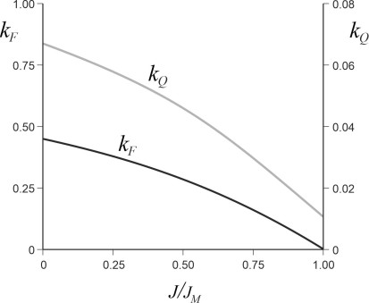
Figure 3
Performance curves
In the absence of cavitation and shock waves, the thrust coefficient \(k_F\) and the torque coefficient \(k_Q\) for a propeller can be considered as functions of \(J\) only, enabling the designer to judge the propeller’s behaviour from two-dimensional performance curves [10] [1]. A typical plot of the thrust coefficient \(k_F\) against advance ratio \(J\) displays a shallow curve as indicated by the black line in figure 3. In fact the thrust is plotted against the ratio \(J/J_m\), in which the quantity \(J_m\) represents an upper limit to \(J\) as we’ll see in a moment. At zero advance ratio, the thrust is greatest – a ship, for example would be straining against its moorings because of the high angle of attack. With increasing \(J\), the angle of attack decreases and the thrust gradually declines. When \(J\) reaches \(J_m\) the thrust finally reaches zero and the propeller ‘freewheels’: it is moving forward through the water but producing no thrust at all.
The corresponding curve for the torque coefficient is not very different. It starts at a high value and declines steadily with increasing \(J\), but unlike the thrust curve it doesn’t intersect the \(J\)-axis on the right hand side of the graph. The reason is that when the angle of attack reaches zero, the blades are still slicing through the water, and some torque input from the engine is needed to overcome the friction.
What can be learned from these two curves? Any point along the horizontal axis represents a possible operating speed for the propeller. The designer wants to know where the optimum lies, but the curves don’t immediately spell it out: a plot of the propeller efficiency would be more helpful. Note that it is the overall efficiency we are dealing with now, not the ideal efficiency. We can work out an expression for the propeller efficiency as a function of the thrust coefficient \(k_F\), the torque coefficient \(k_Q\), and the advance ratio \(J\). The expression we are looking for is the proportion of the power input that is usefully converted into vehicle motion. By definition, the input power is given by the torque multiplied by angular velocity - the speed of rotation in radians per unit time - so that if \(Q\) denotes the torque and \(n\) denotes the number of revolutions per unit time:
(36)
\[\begin{equation} \text{Input power} \quad = \quad 2 \pi nQ \end{equation}\]The output power is just the thrust times the advance speed:
(37)
\[\begin{equation} \text{Output power} \quad = \quad V_{a}F \end{equation}\]and the propeller efficiency is just the ratio of these two:
(38)
\[\begin{equation} \eta \quad = \quad \frac{\text{Useful output power}}{\text{Input power}} \quad = \quad \frac{V_{a}F}{2 \pi nQ} \end{equation}\]We can now substitute for \(F\) and \(Q\) using equations equation 25 and equation 27 to get:
(39)
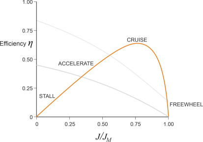
\[\begin{equation} \eta \quad = \quad \frac{V_{a} \left( k_{F} \rho n^{2} D^{4} \right) }{2\pi n \left( k_{Q} \rho n^{2} D^{5} \right) } \quad = \quad \frac{1}{2\pi }\frac{k_F}{k_Q}J \end{equation}\]Hence, the overall efficiency is proportional to \(J k_F/k_Q\), and from the curves of the thrust coefficient \(k_F\) and the torque coefficient \(k_Q\) shown earlier in figure 3, we can picture the curve of overall efficiency against \(J\) as shown in figure 4. The efficiency starts at zero – if there is no advance, the vehicle is stationary and although the propeller is delivering thrust, it is doing no useful work. However, \(\eta\) rises as the advance ratio increases, peaking at a specific combination of torque and thrust. At the right hand side of the graph we see that it falls to zero again, and the fall is quite rapid as the advance ratio approaches the upper end of its range. An aircraft propeller behaves in a similar way. The curve broadly reflects the four operating conditions described in the previous Section: stall, acceleration, cruise, and freewheel (see Figure 15 in Section F1513). Obviously the designer wants the vehicle cruising speed to coincide with peak propeller operating efficiency, at which point the power delivered to the vehicle is obtained at the least possible fuel cost.
However, there is a complication. As it stands, the curve is based on equation 39, which does not take into account the fact that the performance of a ship’s propeller is affected by its position, being mounted close to the stern inside the fluid boundary layer. For a ship, equation 39 measures the ‘open water efficiency’ \(\eta_o\) of the propeller as if it were operating in isolation [5], and we’ll need to adjust the efficiency values to account for the interaction between propeller and hull.
Figure 4
Propeller-hull interaction and its effect on efficiency
In fact the propeller and a ship’s hull interact in two distinct ways. First, the propeller draws water towards it by lowering the fluid pressure in the region ahead, underneath the hull. The reduced pressure has an unwanted side-effect: it acts like a drag force on the hull plating (figure 5). For accounting purposes, the drag can be viewed as a reduction in the propeller thrust and quantified in terms of the thrust reduction factor \(t\) [7] [10]. Assuming that \(t\) can be estimated, it is possible to account for the propeller-hull interference as an incremental reduction in the ‘hull efficiency’ by the factor \((1-t)\).
Figure 5
Second, the propeller disc lies partly or wholly within the hull boundary layer. We’ve already noted that the relative velocity \(V_{\text{in}}\) of the fluid particles approaching the propeller disc is less than the speed \(V\) of the ship through the surrounding water, being reduced by viscous friction within the boundary layer. This should be helpful, because any reduction in \(V_{\text{in}}\) enables a similar reduction in the downstream velocity \(V_{\text{out}}\) without any change in the thrust, meaning that less energy is wasted in the slipstream. The velocity reduction is conventionally represented [4] [10] by the ‘Taylor wake fraction’ \(w_T\) given by :
(40)
\[\begin{equation} w_T \quad = \quad \frac{V-V_a}{V} \end{equation}\]The boundary layer effect can then be expressed as a second adjustment factor equal to \(1/(1-w_T)\). Putting this together with the thrust reduction adjustment factor we get an expression for a quantity known as the ‘hull efficiency’ \(\eta_{\text{h}}\) [3] [10] [16]:
(41)
\[\begin{equation} \eta_h \quad =\quad \frac{1-t}{1-w_T} \end{equation}\]For ships, a further issue arises with the non-uniform nature of the flow across the actuator disc; as explained in Section M1410, it is non-uniform partly because the stream tube tends to be angled upwards slightly and partly because the fluid in the upper half of the actuator disc is entrained within the boundary layer and moves more slowly than the fluid passing through the lower half. As a result, a propeller blade meets different conditions during each revolution as it progresses round its \(360^{\circ}\) orbit, with the thrust on each blade rising and falling more than once during each cycle. The average thrust differs slightly from the figure that would arise in a uniform flow field, and the difference is reflected in the value of the ‘relative rotative efficiency’ \(\eta_r\), which usually lies within the range 0.96 to 1.04 [7].
Overall efficiency
Finally, we can assemble the various adjustment factors into an expression for the overall efficiency of a ship’s propeller [7] [10]; it is called the quasi-propulsive coefficient and since there doesn’t seem to be a standard notation we’ll denote it simply by \(\eta\):
(42)
\[\begin{equation} \eta \quad = \quad \eta_{o}.\eta_{h}.\eta_{r} \end{equation}\]As we saw earlier in figure 4, the open water efficiency \(\eta_{o}\) of a ship’s propeller reaches a peak at a certain operating speed, and when adjusted according to equation 42, presumably the overall efficiency follows a similar profile. For a conventional fixed pitch propeller the optimum efficiency is achieved at a small angle of attack, and from published data, the maximum value for merchant vessels with two or more screws typically falls within the range 60 – 70%, and for single-screw vessels from 70% to over 80% (see, for example, [9] [15] [19]). Over its lifetime, the cost of fuel consumed by a merchant vessel is typically greater than its capital cost, which may well exceed $100 million, so a small percentage improvement in propeller efficiency will represent a significant saving for the owner. By comparison, aircraft propellers seem to be more efficient, typically \(80\) – \(90\%\) [2] [14].
Matching the propeller to the vehicle
An engine works best at a certain speed. Its efficiency peaks when the output shaft is turning at a certain rate and delivering a certain torque, at which point the engine consumes the least possible amount of fuel per kilowatt output (and probably generates the least possible exhaust pollution too). Much the same applies to the propeller. It runs most efficiently at a certain speed of rotation, at which point it wastes the smallest possible proportion of engine power in fluid friction and in churning up the fluid slipstream. Putting these two factors together, the designer tries to match the propeller to the vehicle so they both run at optimum efficiency when the vehicle reaches cruising speed.
It’s common practice to describe the matching problem as one of power absorption – the propeller must be capable of handling the power output from the engine. To understand what this means in practical terms, it may help to express the problem in a different way. Imagine a ship that is now being built. The engine is installed but it doesn’t yet have a propeller. The owner wants to try out three alternatives that we’ll call respectively propellers A, B and C. The first has a shallow pitch so when the ship puts out to sea and the captain calls for full speed ahead, the propeller runs smoothly at a low angle of attack without delivering much thrust: it can’t move the ship forward at its target cruising speed. Meanwhile the engine is racing at its maximum allowable rpm, and since it doesn’t encounter a heavy load, it must be throttled back to avoid being damaged – it’s not working at its full capability. In nautical parlance, the propeller is ‘too easy’.
So the owner removes it and installs propeller B instead. Its pitch is much larger, so when the engine throttle is opened, there is considerable resistance from the propeller blades, which are set at a high angle of attack. The propeller rotates slowly while the engine is labouring at an uncomfortably low rpm: the propeller thrust falls short and again the ship fails to achieve its target cruising speed. The propeller is ‘too stiff’. So the owner replaces it with propeller C, whose pitch lies between that of propeller A and propeller B. At this point, the propeller harnesses all the available engine power to move the ship at its target cruising speed, and it does so at its most efficient speed of rotation so the minimum proportion of energy is wasted. At the same time, the engine is working at peak efficiency too. To summarise, the owner has found a propeller (a) whose power absorption matches the engine power output, (b) that does so when both the propeller and engine are operating at their most efficient speed, and (c) that generates the required thrust. To arrive at this point may require several iterations round a ‘design loop’ as described in [8]. There is no simple formula for determining the optimum shape, and the designer will analyse different profiles and choose the one that works best.
What is going on here?
In figure 6, you can see Brian Kahrs of Clearwater, Florida, riding a vehicle he designed and built himself. Under his right arm he holds a leaf-blower, which provides thrust like a rocket engine. In his left hand he holds an umbrella. One might expect the umbrella to increase the frontal area and therefore the drag, but more important is the exhaust jet of the leaf-blower, which is pointing in the wrong direction. Yet Brian is travelling forward - pretty fast. Can you explain what is going on?
Figure 6

Appendix: Energy wastage and propeller size
Axial momentum theory points to the conclusion that other things being equal, a large, slowly turning propeller is more efficient than a small one turning more quickly, because it transfers less energy into the fluid slipstream. It is common practice to use the ideal efficiency \(\eta_{\text{ideal}}\) as a tool to explore issues of this kind, because in a compact form, it quantifies the energy usefully converted into thrust as a proportion of the total energy supplied by the propeller. Here, we are more interested in a related quantity, \(1- \eta_{\text{ideal}}\), which denotes the proportion of energy that is wasted in the slipstream. We want to know how it varies when we change the size of the propeller by some specified amount; for example, does a small increase in propeller size result in a large reduction, or a negligible one? We shall approach the problem using elementary calculus, which will enable us to estimate the energy saving that arises from an incremental change (say, 1%) in the area \(A\) of the disc.
We start by sketching in a missing detail, the fluid velocity \(V_{\text{disc}}\) through the propeller itself. Assuming that within the stream tube, any radial component of fluid velocity is small enough to be ignored, one can apply Bernoulli’s Principle to the fluid flow between station G upstream and station H as shown in figure 1 to obtain:
(43)
\[\begin{equation} p_{0} + \frac{1}{2} \rho V_{\text{in}}^{2} \quad = \quad p_{\text{f}} + \frac{1}{2} \rho V_{\text{disc}}^{2} \end{equation}\]Similarly for the flow downstream between station I and station J:
(44)
\[\begin{equation} p_{\text{r}} + \frac{1}{2} \rho V_{\text{disc}}^{2} \quad = \quad p_{0} + \frac{1}{2} \rho V_{\text{out}}^{2} \end{equation}\]Adding these two equations together and re-arranging, we get
(45)
\[\begin{equation} p_{\text{r}} - p_{\text{f}} \quad = \quad \frac{1}{2} \rho \left( V_{\text{out}}^{2} - V_{\text{in}}^2 \right) \end{equation}\]If we now multiply the left-hand side by the disc area \(A\) we get the thrust \(F\), therefore
(46)
\[\begin{equation} F \quad = \quad A \left( p_{\text{r}} - p_{\text{f}} \right) \quad = \quad \frac{1}{2} \rho A \left( V_{\text{out}}^{2} - V_{\text{in}}^2 \right) \end{equation}\]But \(F\) also appears on the left-hand side of the elementary thrust equation, originally set out as equation 7:
(47)
\[\begin{equation} F \quad = \quad \rho A V_{\text{disc}} \left( V_{\text{out}} - V_{\text{in}} \right) \end{equation}\]Equating the right-hand side of equation 46 with the right-hand side of equation 47 and cancelling the common factors, we get:
(48)
\[\begin{equation} V_{\text{disc}} \left( V_{\text{out}} - V_{\text{in}} \right) \quad = \quad \frac{1}{2} \left( V_{\text{out}}^{2} - V_{\text{in}}^2 \right) \end{equation}\]which can be simplified to yield
(49)
\[\begin{equation} V_{\text{disc}} \quad = \quad \frac{1}{2} \left( V_{\text{out}} + V_{\text{in}} \right) \end{equation}\]In other words, the velocity of the fluid passing through the propeller disc is the arithmetic mean of the velocities upstream and downstream (we could have guessed this, but a mathematically convincing demonstration takes longer). Now assume that the input velocity is numerically equal to the vehicle’s forward speed \(V\). Since we earlier defined the ‘inflow factor’ \(a\) as half the proportional change in fluid velocity between the upstream and downstream stations G and J, it follows that the downstream velocity is \((1+2a)V\), and we can write
(50)
\[\begin{eqnarray} V_{\text{in}} \quad & = & \quad V \\ V_{\text{disc}} \quad & = & \quad (1+a) V \\ V_{\text{out}} \quad & = & \quad (1+2a)V \end{eqnarray}\]Substituting these three expressions into equation 47 leads to
(51)
\[\begin{equation} F \quad = \quad 2 \rho A V^{2} a(1+a) \end{equation}\]We can now focus on the problem in hand, starting from this new version of the elementary thrust equation. We’ll need some help from equation 12, which tells us that \(\eta_{\text{ideal}} = 1/(1+a)\), so that solving for \(a\):
(52)
\[\begin{equation} a \quad = \quad \frac{1 - \eta_{\text{ideal}}}{\eta_{\text{ideal}}} \end{equation}\]which when substituted in equation 51 yields
(53)
\[\begin{equation} F \quad = \quad 2 \rho A V^{2} \left( \frac{1 - \eta_{\text{ideal}}}{\eta_{\text{ideal}}^2} \right) \end{equation}\]which after rearranging becomes
(54)
\[\begin{equation} \frac{\eta_{\text{ideal}}^2}{1 - \eta_{\text{ideal}}} \quad = \quad \left( \frac{ 2 \rho V^{2}}{ F } \right) A \end{equation}\]The term in braces on the right-hand side is a constant, which we’ll denote by \(C\). We can now use equation 54 to quantify the effect of propeller size on energy wastage. By definition, when expressed as a proportion of the energy supplied by the propeller, the energy wasted in the slipstream equals \(1 - \eta_{\text{ideal}}\). If we denote this quantity by \(\epsilon\), we can substitute \(1-\epsilon\) for \(\eta_{\text{ideal}}\) on the left-hand side of equation 54 to get
(55)
\[\begin{equation} \frac{\left( 1 - \epsilon \right)^2}{\epsilon} \quad = \quad C A \end{equation}\]Now differentiate both sides with respect to \(A\); after tidying up we find that
(56)
\[\begin{equation} - \frac{\left( 1 - \epsilon^2 \right)}{\epsilon^2} \frac{d\epsilon}{dA} \quad = \quad C \end{equation}\]From equation 55 it is clear that \(C = (1-\epsilon)^{2}/\epsilon A\). Substituting this expression for \(C\) on the right-hand side of equation 56, we obtain
(57)
\[\begin{equation} - \frac{\left( 1 - \epsilon^2 \right)}{\epsilon^2} \frac{d\epsilon}{dA} \quad = \quad \frac{ \left( 1-\epsilon \right)^2}{ \epsilon A } \end{equation}\]After simplification, this can be written:
(58)
\[\begin{equation} \frac{A}{\epsilon} \frac{d \epsilon}{d A} \quad = \quad -\frac{ 1-\epsilon}{ 1 + \epsilon } \quad = \quad -\frac{\eta_{\text{ideal}}}{ 2 - \eta_{\text{ideal}}} \end{equation}\]which is the relationship we seek.
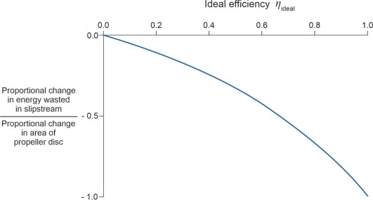
What does this mean in practice? In everyday language, if you increase the area of a propeller disc by a small increment, say \(1 \%\), the energy wasted in the slipstream will fall by \(\eta_{\text{ideal}} / \left( 2 - \eta_{\text{ideal}} \right) \%\). Imagine you have a propeller whose ideal efficiency is 80%, and you’re thinking of replacing it with a slightly larger one. If the disc area of the new propeller is 1% larger than the old one, the pay-off, the fall in wasted energy, will amount to [0.8/(2 - 0.8)] = 0.67% approximately. We’re assuming here that the operating conditions remain unchanged, including the speed of the vehicle, the thrust, and the power delivered to the propeller, so we are comparing like with like. However, as shown in figure 7, the pay-off varies with the ideal efficiency of the original propeller. Two points are worth noting. First, the ratio of the percentage change in wasted energy to the percentage change in \(A\) always lies in the range between -1 and zero, so the pay-off in numerical terms is always less than the change in disc area. Second, the pay-off for an inefficient propeller is smaller than the pay-off for an efficient one. Perhaps this explains why the propellers of small boats such as leisure craft tend to be less efficient than the propellers for larger commercial vessels.
Figure 7
Acknowledgement
Figure 6 Brian Kahrs’ air-propelled vehicle: available at https://www.youtube.com/watch?v=C5EVRYW1qgc accessed 18 November 2020.