M.1620
Ships make waves
Figure 1
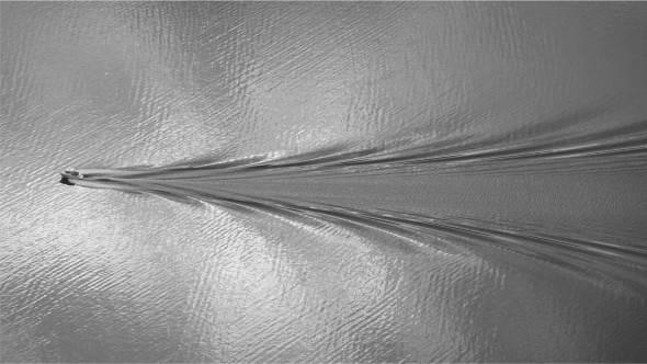
Right now, there are many thousands of ships dotted across the oceans of the world. Each makes a vee-shaped wave pattern on the water surface, a strange and beautiful pattern that’s roughly the same for all ships regardless of their shape or size. The height of the waves and the spacing between them grows with increasing speed, but the geometry is fixed with the same angle of vee throughout. In fact, the pattern is almost identical to the one made by a rowing boat, or a duck paddling across the pond in your local park. The arms of the vee are not single waves but groups of waves in echelon formation. Each wave follows slightly behind and to one side of its predecessor, its height peaking some distance away from the ship as though being towed along by an invisible force. Other waves lie transversely across the ship’s wash between the arms of the vee, and although less prominent, they cover a large area and contain a great deal of energy - it’s the energy put into these waves that accounts for much of the fuel consumed by a ship’s engines as they overcome resistance to motion through the water. In this section we’ll try to understand how the waves are formed, why they take on the shape they do, and ultimately how they limit the speed at which a conventional ship can travel.
Wave formation
Let’s start with a broader question. How does a wave form, and how does it move? Earlier in Section M1820, we saw how the wind can raise waves on the water surface. Here, we’re interested in waves caused by a local disturbance such as a stone falling into a pond. The stone displaces water particles, which momentarily form a wall around the cavity left by the stone as it plunges below the surface. The wall then collapses, which disturbs more particles on the water surface on either side. These in turn rise momentarily and then collapse, disturbing yet more particles in the neighbouring ring. Thus, the original ‘wall’ propagates outwards in the form of a circular wave. It also propagates inwards to fill the central cavity, where the particles collide and generate a new disturbance at the core. There follows a complex series of circular waves expanding at different speeds and with different wavelengths across the water surface.
Wave behaviour
In different situations, surface waves behave in different ways, and in Section M1820 we looked at an idealised variety called plane progressive waves. In a regular series of waves, the horizontal distance \(\lambda\) between successive crests is called - not unnaturally - the wavelength, and the height of each crest relative to the mean water level is known as the amplitude, which we’ll denote by \(a\). If the amplitude is small relative to the wavelength, the surface profile closely resembles a sine wave. Technically, the speed at which the shape of the crest travels is known as the phase velocity, but we’ll just call it the velocity. In deep water, for waves of any given wavelength \(\lambda\) , the velocity \(C\) and the wavelength are related by the formula
(1)
\[\begin{equation} C \quad = \quad \sqrt{ \frac{g \lambda}{2 \pi} } \end{equation}\]Among other things, this tells us that long waves travel faster than short ones. We also learned in Section M1820 that waves are not exclusive. Several distinct wave trains, each of different wavelength and travelling in different directions, can occupy the same patch of water at the same time. Imagine an individual wave of amplitude \(a\) arriving at a point P in the middle of a lake. When it reaches P, it will pile on top of all the other waves that happen to be passing through P at that moment, and raise the level by an amount \(a\). It will be followed by a trough immediately behind, which depresses the surface instead. If all the waves passing through P are sine waves of modest amplitude, the elevation of the water surface at any particular moment is just the sum of the elevations of the individual waves, which emerge from the encounter unchanged.
Froude number
Imagine you are sailing a boat across a lake. It is a model boat, scaled down to one hundredth the size of a real steamer. To look realistic, how fast should it sail? Common sense suggests that the distance it covers in any time interval should be scaled down in the same ratio as the length of the model, in other words, the speed should be scaled down by a factor of a hundred. Then, the time taken by the model to move one length forward and the time taken by the real ship to move one length forward would be the same, and if you filmed them both in action and compared the two films, it would be hard to tell which was the model and which was the real steamer.
But what about the wave pattern? During the late 19th century, the mathematically gifted engineer William Froude realised that to simulate the ship’s behaviour correctly, the waves too should scale down in proportion to the size of the hull. Otherwise, the resistance incurred by the model would not accurately reflect the resistance incurred by the ship. Specifically, the ratio of the wavelength to the hull length must be the same in both cases. However, there is a snag. If you scale down the speed in line with the hull length, the wave pattern will be wrong. Equation 1 tells us that the wavelength is proportional to the square of the speed, so the wave pattern will scale down by a factor of \(\left(1/100 \right)^{2}\), reducing its dimensions to a tiny fraction of what they should be. Hence the model must sail a lot faster than its ‘natural’ scale speed.
Imagine the original vessel shrinking bit by bit from its original size. In order for the wavelength to scale down in proportion to the ship’s length \(L\), we see from equation 1 that the wave velocity \(C\) must scale down in proportion to \(\left( gL \right)^{1/2}\), and since the wave pattern is travelling along with the ship, the wave velocity \(C\) at each stage equals to the ship’s velocity \(V\). It follows that \(V\) must be kept proportional to \(\left( gL \right)^{1/2}\), or to put it another way, the ratio \(V/\left( gL \right)^{1/2}\) must remain constant throughout – and ultimately it must have the same value for the model as it does for the original steamer. In particular, our model must sail at a velocity equal to one tenth of the velocity of the steamer, and not one hundredth of its velocity as common sense might suggest.
The ratio \(V/ \left( gL \right)^{1/2}\) has special significance. A dimensionless number, it reduces the motion of all displacement vessels to a common yardstick. Today, it is known as Froude’s number and denoted by the symbol Fr:
(2)
\[\begin{equation} \text{Fr} \quad = \quad \frac{V}{\sqrt{gL}} \end{equation}\]The term \(g\) appears in the denominator because the behaviour of plane progressive waves depends on the strength of the gravitational field. On a more massive planet than the earth, waves of any given length will move more quickly than they do here (and conveniently, putting \(g\) in the denominator turns the Froude number into a dimensionless measure that will have the same value no matter what units you happen to be working in).
In effect, the Froude number is a way of expressing the speed of the ship in relation to the speed of a wave of comparable size. A wave can itself be treated as a moving object whose size is measured by its wavelength \(\lambda\), and like a ship it can be assigned a Froude number. From equation 1 its velocity is \(\sqrt{ g \lambda / 2 \pi{} }\). Substituting this expression for \(V\) in equation 2 together with \(\lambda\) for \(L\), the Froude number for a plane progressive wave comes to \(\sqrt{ g \lambda / 2 \pi{} }\) divided by \(\sqrt{ g \lambda }\), which is just \(\sqrt{ 1 / 2 \pi{} }\). The Froude number for all such waves, regardless of speed or wavelength, is approximately 0.4. Some ships can go faster, at speeds corresponding to Froude numbers greater than 0.4. Later, we’ll learn that the wave pattern they create in the water surface is fundamentally different from the wave pattern for ordinary displacement vessels – in a sense, the waves can’t keep up. Most of the material in this Section applies to ships travelling more slowly than this, typically cargo ships, fishing boats, and pleasure yachts. You’ll find a little more information about the Froude number and its wider role in vehicle dynamics in Section F1817.
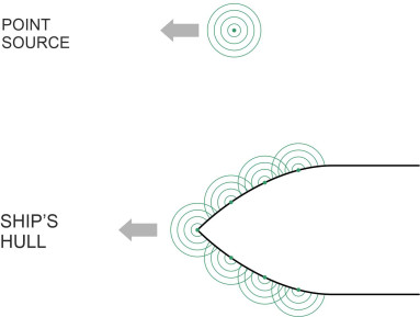
How a ship makes waves
Figure 2
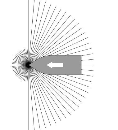
The waves made by a ship are similar to waves moving freely over the ocean. They are created at the interface between two fluids, and they obey the same laws of motion. The difference is that a ship’s waves are not travelling under their own volition as it were, but behave as if connected to the hull (figure 2), trailing along in the ship’s wake and moving at the same speed. How to explain this? During the nineteenth century, the problem attracted the attention of several distinguished scientists. The first to develop a convincing model was William Thomson (later Lord Kelvin) in 1887 [20] [9], although his analysis was developed by others over many decades. They knew that the pattern arises from the superposition of wave trains, which reinforce each other in some places while cancelling each other out in others. It is an ‘interference pattern’, similar in principle to those that occur in optical experiments in which light beams are combined to form geometrical patterns on a flat screen. A ship’s wave pattern is more complicated because (a) the pattern is moving, and (b) it is the result of many wave trains emanating from different points along the ship’s path. It’s not easy to predict what the pattern looks like, but there are two ways of doing it. The first is to draw a large number of individual wave trains and trace out their envelope on a piece of paper. The second is a mathematical method, which (essentially) identifies locations in the ship’s wake where the individual wave trains reinforce each other, and traces the loci of the crests. In what follows, we’ll start with the graphical method, and then briefly describe the analytical method and plot some results.
Geometry of the wave pattern
For the moment, we’ll concentrate on the bow of the ship and ignore anything that might be happening astern. We treat it is a moving ‘pressure point’. Deep under water, the bow pushes fluid aside, creating a region of high pressure that extends upwards to the waterline and forces some of the water particles to rise and spill over onto the surface. The effect is rather like a series of boulders falling one by one into the water at each location along the ship’s path, simulating a continuous disturbance that progresses along the surface with velocity \(V\), and creates waves that propagate into the surrounding area. One might expect them to spread out in circles around all points of the compass, but interestingly, nothing appears in the water ahead of the bow. Instead, when superimposed, the wave-circles produce a different pattern that is confined to a narrow vee in the ship’s wash.
Graphical construction
We’ll start by constructing the wave pattern using a graphical method. It involves very little mathematics: instead we picture each crest as a superposition of the wave-circles generated along the ship’s path, and as if by magic, the wave pattern emerges from their envelope. The method was first employed by a contemporary of Thomson’s, Lord Rayleigh (William Strutt), who was interested in the pattern made by a fishing line trailing in a river [4]. In 1883, he pictured the disturbance where the fishing line entered the water as the combined effect of ‘pressure lines’ located on the water surface, all plotted as straight lines passing through the entry point at different angles to the direction of flow. However, readers might find the approach used here easier to understand, because it’s based on circular waves of the kind we see when a stone falls into a pond. In the end, we’ll arrive at the same result, although it will take us longer to get there.
Figure 3
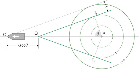
Let’s start by assuming that the ship is following a straight course so the bow cleaves the water surface at a steady speed \(V\). We’ll adopt a frame of reference that is moving along with the ship, with the x-axis aligned opposite to the direction of motion, and the y-axis at right-angles to it, positive to starboard. At each point, the bow generates many wave-circles that radiate outward, each of a specific wavelength \(\lambda\), and phase velocity \(W\) given by
(3)
\[\begin{equation} W \quad = \quad \sqrt{ \frac{g \lambda }{2 \pi} } \end{equation}\]An example of such a wave-circle is shown in figure 3. Its life begins when the ship’s bow O arrives at a particular point P in its path, and as seen from the ship, the circle grows in diameter while receding astern.
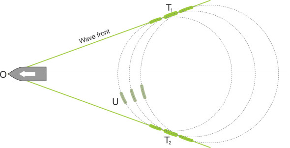
Figure 4
In figure 4, we see the evolution of this wave-circle from the moment of conception. The point T1 lies on the common tangent OT1 that is attached to the ship’s bow at O. Denote by \(\theta\) the angle between the perpendicular PT1 and the ship’s direction of motion. Since the wave-circle expands radially at its phase velocity \(W\) in the direction PT1, it follows that
(4)
\[\begin{equation} W \quad = \quad V cos \theta \end{equation}\]Substituting for \(W\) in equation 3 and rearranging, we see that the wavelength \(\lambda\) of the wave-circle must satisfy the equation:
(5)
\[\begin{equation} \lambda \quad = \quad \frac{2 \pi}{g} {V}^{2} {cos}^{2} \theta \end{equation}\]As the wave-circle grows, the point T1 on its circumference traces out a path along the tangent, creating a wave front that potentially contributes to the ship’s wave pattern on the starboard side as shown in figure 5. Similarly, the point T2 creates a second wave front on the port side. These are the only points on the circumference that can play a part in in the final wave pattern – you can see that the point marked ‘U’ for example does not not trace out a coherent wave front moving along with the ship.
Figure 5
What we’ve just described is how a wave-circle of one particular wavelength plays its part in the ship’s wave-making process. In reality, the bow generates many such wave-circles at each location along its path, each of different wavelength and each expanding at a different rate – in order to determine the ship’s wave pattern, we must picture the effects of all the wave-circles combined, by plotting their tangential wave fronts superimposed on a single diagram. The result appears in figure 6, which shows wave fronts for successive values of \(\theta\) between -90\(^{\circ}\) and +90\(^{\circ}\) at intervals of 5 degrees. There’s not much to see. The wave fronts cross each other at the ship’s bow, where they indicate an intense ‘spike’ but nothing resembling an extended wave crest.
Figure 6
There is of course something missing. Until now, we have been speaking of a wave-circle emanating from a point P as if it were an isolated event. In fact, a wave can’t happen on its own, only as a member of a train of waves of identical wavelength as shown in figure 7. They are spaced radially a distance \(\lambda\) apart. We can number them \(i = 0, 1, 2, ...\) and so on. Think of the first wave-circle to appear as the ‘primary’ or leading member, numbered zero. As we have seen, leading wave-circles contribute to the ship’s wave pattern only at the bow itself. They produce a very localised disturbance. We are more concerned with the trailing waves, principally the ones numbered \(i = 1\) that follow immediately behind. From figure 7 you can see that when the first of these trailing wave-circles begins to form at O1, the ship has moved forward a distance equal to \(\lambda\)sec\(\theta\), and the wave fronts of interest are located on the tangent lines O1T1 and O1T2. Unlike the ones shown in figure 6, these wave fronts pass through a point that lies some distance aft of O.
Figure 7
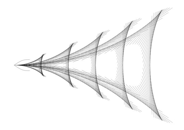
In principle, we can now plot the wave fronts for this particular wavelength and for all other possible wavelengths on the same diagram to obtain the envelope we seek. This time, we plot them for values of the angle \(\theta\) in regular increments of 2.5\(^{\circ}\) between \(-90^{\circ}\) and \(+90^{\circ}\). In each case we use equation 5 to determine the corresponding wavelength and hence the location of the intercept O1 and the tangent point that together define the wave front. The result appears in figure 8. When combined, the wave fronts trace out a curved envelope, which represents the first wave crest that appears in the ship’s wave pattern. You’ll notice that it’s actually a combination of three distinct wave crests. The part of the envelope coloured in red looks as though it has emerged from a separate process, but in fact it hasn’t: for these particular values of \(\theta\) it is aligned in a different way, across the ship’s path, to form what is called a transverse wave. The black lines define diverging waves.
We can now apply the same procedure to the subsequent wave-circles \(i = 2, 3, 4,...\). Each set generates a further wave crest in the ship’s wave pattern. They all have the same shape: for example, the wave crest for \(i = 2\) takes the same geometric form as the first one but is twice the size. The third crest is again identical to the original with its dimensions scaled up by a factor of 3. Figure 9 shows the first five, all superimposed on the one diagram.
Figure 8
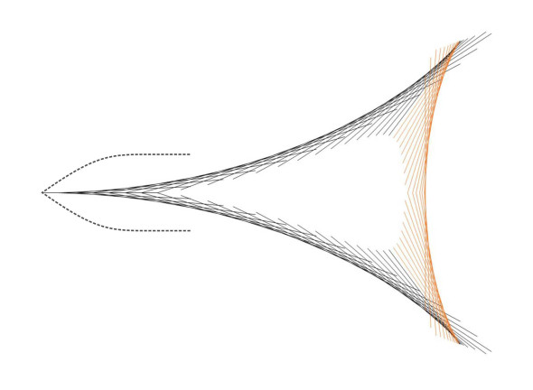
Figure 9
Theoretical derivation
We used a rough-and-ready argument to deduce wave pattern shown in figure 9, but the results compare well with those obtained by William Thompson. In 1887, he was able to trace out the pattern of wave crests in plan view using integral calculus [20]. The analysis involved a technique he had developed called the stationary phase method, which nowadays is used in other areas such as optics and climate science as well as hydrodynamics. The analysis starts by picturing a point Q that lies on the water surface but moves along with the ship, in scientific jargon, a point within a moving field tied to the ship’s frame of reference. Figure 10 shows a wave train arriving at Q having been transmitted earlier when the bow was at P. Others will join it, having been transmitted from different points along the ship’s path to arrive in the neighbourhood of Q at the same time. They will all have different velocities and wavelengths. At places where the peaks don’t coincide there is no reinforcement and no wave. If the peaks reinforce one another and they are moving at the right speed they will make a wave crest that appears to be attached to the vessel.
When Thomson’s loci are superimposed on the envelopes shown in figure 9, the two are indistinguishable. However, Thomson’s method is flawed in the sense that it breaks down at the cusps along the boundary of the vee, where it predicts waves of infinite height. Over the century that followed, other researchers refined his model using essentially the same argument, but modified to iron out the singularities [4]. The maths is not easy to follow, so we won’t work through the derivation here, but instead, try to describe the rationale in everyday terms and quote some key results as set out in [7]. They are reproduced in the Appendix attached to this Section, from which one can work out numerical coordinates for the wave crests on a spreadsheet. Note that the results are asymptotic approximations to the wave pattern ‘in the far field’, meaning that they’re not valid in regions close to the hull.
Figure 10
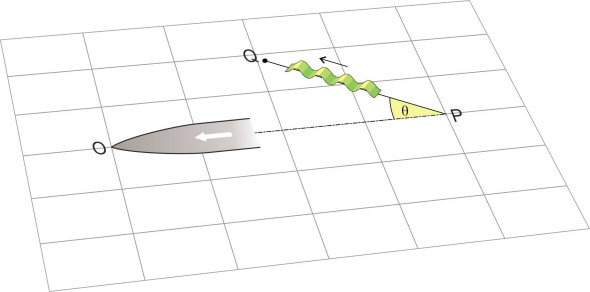
Figure 11
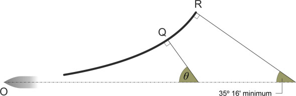
A typical diverging wave crest is shown in figure 11. It is curved in plan. For any particular point Q along the crest, the normal to the crest at that point subtends an angle \(\theta\) with the ship’s course. The highest angle (\(90^{\circ}\)) occurs at O where the crest is parallel to the direction of motion, but the angle falls gradually to a value of \(35^{\circ} 16^{\prime}\) at R where the wave crest terminates at its outer extremity. Like all ship’s waves, each diverging wave is carried along with the hull and hence its velocity is \(V\) when measured parallel to the ship’s course, but when measured at right angles to the crest at any particular point where the normal subtends an angle \(\theta\), the phase velocity is \(V cos \theta\).
Figure 12
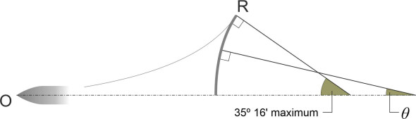
Now for the transverse waves. Although the causal mechanism is exactly the same, transverse waves are associated with values of \(\theta\)below \(35^{\circ} 16^{\prime}\); they are aligned broadly at right-angles to the ship’s course as shown in figure 12. Again, their phase velocity varies according to the angle \(\theta\), but along the ship’s axis where \(\theta = 0\), it is equal to the ship’s own velocity \(V\). If we denote their wavelength measured parallel to the x-axis by \(\lambda_{0}\), then from equation 1 we see that
(6)
\[\begin{equation} \lambda_{0} \quad = \quad \frac{2 \pi V^{2}}{g} \end{equation}\]which is much greater than the wavelength of any diverging wave.
Figure 13
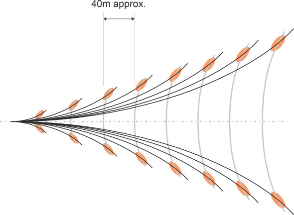
Both sets of waves, diverging and transverse, are plotted in figure 13 for a ship travelling at 15 knots. Notice that the two sets of curves don’t quite marry up. In Thomson’s original drawings, and in figure 9, each diverging wave meets its corresponding transverse wave at a cusp on the boundary of the wave pattern. But here, the two sets are out of phase, the difference being equal to \(\lambda_{0}/4\), and each diverging wave crosses its corresponding transverse wave a little way inside the boundary. The crossing points are highighted in red. Here, the two wave systems reinforce one another, and we expect the elevation to be higher than elsewhere in the wash. In a qualitative sense, this explains the ‘echelon’ waves that figure prominently in the ship’s wash at some distance from the hull.
Figure 14
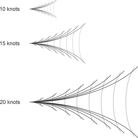
Finally, the spacing between all the waves in the wash varies with the ship’s speed. For example, when measured along the centreline of the ship’s path, the transverse waves are spaced one wavelength apart, and their wavelength, as specified by equation 6, is equal to \(2 \pi V^{2}/g\). It follows that when measured longitudinally, the spacing between all the waves scales up and down in proportion to the square of the ship’s velocity (figure 14).
The Kelvin angle
From a distance, a ship’s wave pattern looks V-shaped because all the ship’s wash is contained within an angle of about 19.5º on either side of the direction of motion: the so-called ‘Kelvin angle’ \(\alpha_{c}\) (figure 15). To find the Kelvin angle, suppose the bow pressure point moves from P to O in a straight line at constant speed \(V\) over a time interval \(t\) as shown in figure 16. The distance covered is \(Vt\). Consider the energy put into the ship’s waves through impulses originating at P. We know that a wave train emitted at angle \(\theta\) to the direction of motion will contribute to the ship’s wave pattern only if its phase velocity equals \(V cos \theta\). Also, as explained earlier in Section M1820, the speed at which wave energy propagates is half the phase velocity, so that in time \(t\) the energy will have travelled a distance \(V t cos \theta /2\). Hence the energy radiated from point P will be contained within the area bounded by the red line in figure 16, whose locus is a semi-circle of diameter \(Vt/2\) centred on the point C, which in turn is located at a distance \(Vt/4\) upstream of P. Energy fronts radiated from other points P1, P2, ... also take the form of semicircles. The envelope is defined by the common tangent to all these semicircles.
Figure 15
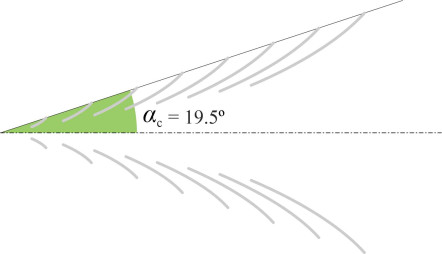
Figure 16
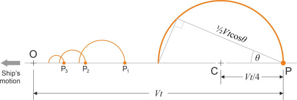
Figure 17
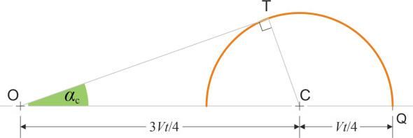
Now let’s return to the original semicircle, which is pictured again in figure 17. If the common tangent meets this semicircle at T, then the tangent together with the radius CT and hypotenuse OC together form a right-angled triangle, with the angle TOC equal to the Kelvin angle \(\alpha _{c}\). Hence
(7)
\[\begin{equation} \sin \alpha_{c} \quad = \quad \frac{ \frac{1}{4} Vt }{ \frac{3}{4} Vt } \quad = \quad \frac{1}{3} \end{equation}\]from which \(\alpha_{c} \sim 19.5^{\circ}\). No wave activity can take place outside this angle. It is the same for all ships travelling in deep water at speeds corresponding to a Froude number of less than about 0.4.
Real ships
It’s striking how the wave pattern emerges from geometric reasoning, without any reference to the physical properties of water. The vessel could be sailing across a sea of liquid methane on one of Saturns’s moons – the mathematics tells us that it would leave a trail of waves like the ones we see here on earth. It also tells us that wherever the ship is sailing, the pattern doesn’t vary with the shape or size of the hull, which could be a 400 m-long container vessel, a model boat only 400 mm long, or even a duck paddling in your local pond. It’s a universal phenomenon.
But is this actually what happens? Let’s look again at the assumptions on which the analysis is based. First, we’ve assumed that the ship is sailing in deep water, that the water behaves as an ‘ideal fluid’ with no friction among the water particles, and that all the waves involved are of modest amplitude. Then, to a close approximation, the profile of each wave follows a sine-curve, and it can be shown that under these circumstances, its wavelength and velocity are related according to equation 1. You’ll notice that neither the density nor the viscosity of the fluid appears in this equation, or indeed in any of the equations set out in the Appendix, so in theory, the wave pattern is the same for any fluid.
Figure 18

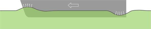
However, when travelling at cruising speed, a ship will generate wave-circles of greater amplitude than this model assumes, especially close to the bow. Here, we observe that the sharp change in pressure triggers a wave that locally is too steep to be sustained. At moderate speeds corresponding to a Froude number around 0.25, the wave curls over and breaks (figure 18); it also generates a greater or lesser amount of spray [1]. The shape of the bow affects the wave pattern in another way too. Until now, we have pictured the hull as a point disturbance whereas in reality, it is a three-dimensional body with curved ‘entrance’ and ‘run’. Hence the wave patterns sketched out in figure 8, figure 9 and figure 13 can apply only to regions at an appreciable distance from the ship. Closer in, the fluid motions are more complex. If we notionally divide the hull plating on either side of the bow into vertical strips, we can picture each strip as a separate vertical ‘rod’ or point disturbance as shown in figure 19 – we have, in fact, a wall of rods arranged around the waterline, each generating its own wave-circles. The effect is to modify the wave pattern close to the design waterplane. By contrast, the sides of the hull are roughly parallel to the direction of motion, so they slide through the water with minimal disturbance. This is not true of the ship’s stern. Like the bow, it can be pictured as a pressure point, and it creates waves in a similar way. But they are of opposite phase, because the stern pressure point is negative - it sucks water in from behind. Moreover, the hull has finite width and where it curves inward towards the rudder, the plating acts like a ‘wall’ of (negative) point disturbances each generating wave-circles that complicate the basic pattern. So in reality, the bow wave pattern and the stern wave pattern of a real ship may be a little different from the ones we have predicted: broadly similar overall, but differing locally depending on the shape of the hull. Furthermore, in what follows we’ll see that the two wave patterns interact in a way that affects the ship’s resistance.
Figure 19
Wave-making resistance
Although the geometry is interesting, what really matters is that a ship’s waves absorb energy, and the energy loss implies resistance to motion. The energy that a wave carries, per unit area of water surface measured in plan, is proportional to the square of the amplitude, so tall waves are much more energetic that shallow ones. On this basis, you’d expect the diverging waves to play the dominant role here, but in fact it’s the other way round. Even though they have relatively low amplitude, it’s the transverse waves that absorb most of the energy, because each covers a large area and contains a great deal of water.
Energy flow
Once a ship reaches cruising speed, the hull continues to pump energy into the wash at a constant rate, and in open water, the area covered by the wave pattern grows steadily over time. The rate of growth is fixed, because the energy in a wave train travels at half the phase velocity of the individual wave crests, so if the ship’s cruising speed is \(V\), the energy lags behind at velocity \(V/2\), with new wave crests appearing almost magically at regular intervals at the rear edge. Each fits into the angle of the vee and (as measured perpendicular to the \(x\)-axis) is wider than its predecessor and covers a greater area. But it carries the same amount of energy, hence the amplitude of successive waves declines steadily from front to rear.
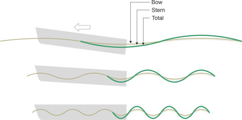
Using the mathematical models created by Thomson and his successors, scientists have tried to predict the wave amplitudes and work out the implications for a ship’s resistance to motion. However, there is a complication: a ship creates two wave systems, one attached to the bow and the other to the stern, and they interact with one another in the ship’s wash.
Interaction between the bow and stern systems
A ship’s stern creates waves in much the same way as the bow, except it behaves as a ‘suction point’ drawing water particles inwards rather than pushing them away. In a sense, it’s a negative version of the bow that creates waves of opposite phase (figure 20). The bow waves and the stern waves overlap in the ship’s wash, and before going any further we need to understand how they might interact. There are differences of opinion about exactly where either system can be said to be anchored to the hull, but for the purpose of analysis the distance between the two anchor points is often taken as \(90\%\) of the overall length of the hull measured at the waterline, a distance known as the characteristic hull length. Each system contains a series of peaks and troughs at regular intervals. The bow system starts with a peak whereas the stern system starts with a trough, but their wavelengths are identical. If the peaks of the bow wave system coincide with the peaks of the stern wave system, they tend to reinforce one another. On the other hand, if the peaks of the bow wave system coincide with the troughs of the stern wave system, they tend to cancel each other out. Reinforcement implies bigger waves, greater loss of energy, and greater resistance, whereas cancellation means that less energy is wasted and the resistance to motion is reduced.
Figure 20
As we’ll see in the next Section, there are other forms of resistance, all of which are related to the ship’s velocity \(V\) in a simple way: they increase roughly as \(V^{2}\). If there were no interaction between the bow and stern wave systems, one might expect the wave-making resistance to behave likewise: it should rise smoothly as the square of velocity in the same way. But given that the wavelength varies with speed, it appears that the degree of interaction can rise and fall abruptly depending on how fast the ship is travelling, and the resistance curve will rise and fall with it. It is not difficult in principle to determine the location of these ‘humps’ and ‘hollows’.
Good and bad Froude numbers
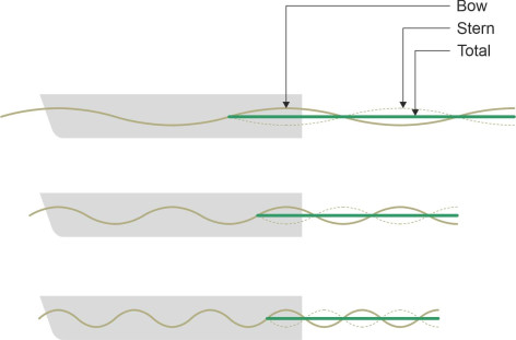
All we need to do is look at the train of waves produced by the bow: does it have a peak or a trough at the stern? Three specific cases are shown in figure 21. In the first case, the wavelength \(\lambda\) of the bow system is twice the length of the ship, so that its first trough coincides with the initial trough of the stern system. The two reinforce, so the amplitude of the combined wave is greater than the amplitude for either wave system on its own. Under these conditions, the wave-making resistance rises to a peak often called the ‘main hump’. If we take the distance between the bow wave system and the stern system as around 0.9 times the waterline length \(L\) of the ship as described earlier, then
(8)
\[\begin{equation} \lambda \quad = \quad 2 \times \left( 0.9L \right) \end{equation}\]Figure 21
Denoting the ship’s speed by \(V\), from equation 1 we have that
(9)
\[\begin{equation} \lambda \quad = \quad \frac{2 \pi V^2}{g} \end{equation}\]If we substitute the right-hand side of equation 8 for \(\lambda\) and re-arrange we get
(10)
\[\begin{equation} \frac{V^2}{gL} \quad = \quad \frac{0.9}{\pi} \end{equation}\]which implies that:
(11)
\[\begin{equation} \text{Fr} \quad = \quad \sqrt{\frac{0.9}{\pi}} \quad = \quad 0.54 \end{equation}\]The next peak occurs when the wavelength is equal to 2/3 times the characteristic hull length as shown in the second of the three diagrams that appear in figure 21. It is called the ‘prismatic hump’. Other peaks are less noticeable – they occur when the wavelength is 2/5 times the characteristic hull length, 2/7 times, and so on, in other words
(12)
\[\begin{eqnarray} \lambda \quad = \quad \frac{ 2 \times \left( 0.9L \right)}{2i+1} & (i\; = \;1,\;2,\;3,...) \end{eqnarray}\]The corresponding Froude numbers are given by
(13)
\[\begin{equation} \text{Fr} \quad = \quad \sqrt{ \frac{0.9}{(2i+1) \pi }} \end{equation}\]The results are summarised in table 1. The numbers in the right-hand column are what you might call unfavourable Froude numbers that the ship owner would prefer to avoid. They are numerically the same as the ones cited by [18], and also by [17] using a different notation, but they differ slightly from those appearing in [3] and [7], which are based on different assumptions about the location of the interacting wave systems relative to the hull.
| \(i\) | \(\lambda / (0.9\textit{L})\) | Fr | |
| 0 | 2 | 0.54 | Main hump |
| 1 | 2/3 | 0.31 | Prismatic hump |
| 2 | 2/5 | 0.24 | |
| 3 | 2/7 | 0.20 | |
| 4 | 2/9 | 0.18 |
In the same way, one can highlight the wavelengths and Froude numbers where the bow and stern systems tend to cancel out - these produce local reductions or ‘hollows’ in the resistance curve and point to favourable operating conditions. The wave forms are shown in figure 22, and the details set out in table 2.
Figure 22
| \(i\) | \(\lambda / (0.9\textit{L})\) | Fr | |
| 1 | 1 | 0.38 | Prismatic hollow |
| 2 | 1/2 | 0.27 | |
| 3 | 1/3 | 0.22 | |
| 4 | 1/4 | 0.19 |
The resistance profile
The effect on the curve of resistance against operating speed varies from vessel to vessel and is sensitive to variations in the shape of the hull. A hypothetical representation of the curve is shown in figure 23. At low speeds, the wave-making resistance is small (it’s actually swamped by friction [8]). There follows an irregular series of humps and hollows before the curve bottoms out in the prismatic hollow at a Froude number of about 0.38, highlighted in green in the Figure. For many vessels this represents an ideal operating speed. Above a Froude number of 0.4, the maximum value at which conventional displacement ships are designed to operate [16], the curve rises quickly towards the right-hand side of the graph, where at a Froude number of 0.5, wave-making dominates other sources of resistance. In principle, the curve should continue to rise thereafter, but what actually happens is that for speeds in this region, the vessel begins to plane. At this point, the wave-making resistance falls again as other forms of resistance take over.
Figure 23
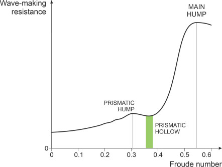
In the Figure we have made the humps and hollows small, because it seems that for real ships, they are less pronounced than our simplified model would suggest [14]. There are at least two possible reasons for this. First, the stern system fits inside the envelope of the bow system in such a way that none of its transverse waves can totally reinforce or totally cancel the corresponding bow wave. Second, as mentioned earlier, both the bow and the stern have finite width and behave as multiple point disturbances. These disturbances blur the wave pattern and weaken the interaction.
Theoretical hull speed
Let us return to the ‘main hump’ mentioned earlier. Although the resistance profile varies from ship to ship, in most cases the main hump is a prominent feature. It corresponds to the worst possible condition in which the wavelength of the disturbance at the bow and the wavelength of the disturbance at the stern are both equal to twice the waterline length of the ship. As shown in the uppermost diagram in figure 21, the two wave systems reinforce so that the bow of the ship is supported by a crest while the stern sinks into a trough. The ship squats deeper in the water with the bow angled upward as if travelling uphill. This condition represents a practical limit for a conventional displacement vessel because it will need a great deal more power to make it go any faster [15]: at this point it is said to be travelling at its theoretical hull speed. Assuming that the characteristic length is 90\(\%\) of the waterline length, the Froude number is about 0.54, so the theoretical hull speed is given by
(14)
\[\begin{equation} V_{\text{theoretical}} \quad = \quad 0.54 \sqrt{gL} \end{equation}\]This formula explains why other things being equal, large ships are faster than small ones. If you double the hull length L, equation 14 tells you that the theoretical hull speed will increase by about 40\(\%\). For economic running, displacement vessels are designed to operate at a lower Froude number of about 0.35 [15]. This corresponds to a lower resistance value in the ‘prismatic hollow’: the wavelength is roughly equal to or a little greater than the characteristic hull length so the bow waves and stern waves tend to cancel out [17]). For other vessels such as surface-effect ships and hovercraft, the humps and hollows are located in different places along the resistance profile because the degree of interference between the bow and stern wave systems is sensitive to other factors [2] [8].
Wave patterns at higher speeds
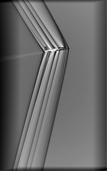
So far we have been dealing with displacement vessels that move relatively slowly in deep water, such as cargo ships, passenger liners, and the like. The waves they make are confined within a vee-shaped boundary, while outside the boundary they create little or no disturbance on the water surface. This pattern reminds one of the shock wave created by an aircraft flying at supersonic speed as shown in figure 24, a ‘schlieren photogaph’ of a US Air Force jet trainer. However, there are differences. First, a supersonic shock wave is three-dimensional, and the air passing through it undergoes compression. By comparison a ship’s wave is just a two-dimensional surface at the interface between two fluids, and the water passing through it doesn’t undergo compression. Second, as the speed of the aircraft increases, the compression becomes more severe and the angle of the vee falls. For a ship’s wave, on the other hand, given that the Froude number is less than 0.4, the angle of the vee remains constant. Nevertheless, fast ships can create wave patterns that in some respects do resemble a shock wave, particularly in coastal areas where the water is shallow.
Figure 24
Shallow water
It well known that in shallow water, waves move more slowly than they do in deep water. This applies to all types of wave, including wind-driven waves approaching the coastline, and also the wave-circles made by a moving vessel. More precisely, as the depth \(h\) falls, the phase velocity \(C\) of a freely moving plane wave changes from the value specified in equation 1 to a lower value [12] given by:
(15)
\[\begin{equation} C \quad = \quad \sqrt{\frac{g \lambda}{2 \pi} \tanh \left( \frac{2 \pi h}{\lambda} \right) } \end{equation}\]If you compare the right-hand side of equation 15 with the right-hand side of equation 1 you’ll see that \(C\) is reduced by a factor equal to \(\sqrt{\tanh(2 \pi h / \lambda ) }\). You may or may not be familiar with the function under the square root sign: it is the hyperbolic tangent denoted by \(\tanh(.)\). The value of \(\tanh ( z )\) for any particular exponent \(z\) is equal to \(( e^{z} - e^{-z} )/( e^{z} + e^{-z} )\). For large values of \(z\) its value approaches one, so in deep water where \(h/ \lambda\) is large, \(z\) is large, the reduction factor is unity, and we are back to the original formula in equation 1. For shallow water its value is always less then one, indicating that the waves slow down. In very shallow water, as the ratio \(h/\lambda\) approaches zero, the phase velocity approaches a limit that is independent of wavelength. By expanding the exponential functions in the above expression for \(\tanh ( z )\) as power series in \(z\), it is not difficult to show that for small \(h/ \lambda\), the phase velocity asymptotically approaches the limit \(C_{\text{crit}}\) given by
(16)
\[\begin{equation} C_{\text{crit}} \quad = \quad \sqrt{gh} \end{equation}\]Here the velocity depends entirely on the water depth \(h\), and all waves travel at the same speed irrespective of wavelength. At this point you might be wondering what a reduction in phase velocity has got to do with shock waves: the answer is that since disturbances travel more slowly in shallow water, a fast-moving vessel is more likely to leave its wave pattern behind.
High speed
The crest of a transverse wave forms a shallow curve that straddles the ship’s wash. At the wash centreline, it is perpendicular to the direction of motion and travelling at a phase velocity equal to the ship’s velocity \(V\). You’ll recall that the Froude number of a freely moving plane progressive wave is around 0.4. When the ship reaches a speed such that the Froude number of the hull exceeds 0.4, effectively it is moving faster than the transverse waves – they are left behind, or more correctly, can’t be sustained. This has vital implications for energy dissipation in the vessel’s wash. Normally, most of the energy goes into the transverse waves, and if these waves vanish, all the energy must switch to the diverging wave system. At this point, the ship is said to have reached critical velocity.
Marine engineers distinguish the threshold in terms of a dimensionless parameter similar to the Froude number. It is called the depth-limited Froude number or ‘depth Froude number’ for short. Denoted by \(\text{Fr}_{h}\), its value is given by [6]:
(17)
\[\begin{equation} \text{Fr}_{h} \quad = \quad \frac{v}{ \sqrt{gh}} \end{equation}\]The expression on the right-hand side is the ratio of the ship’s velocity to the fastest speed a wave can travel in a water of depth \(h\), as specified by equation 16. When a ship travels slowly such that the depth Froude number is less 1.0, it is said to be ‘subcritical’. As \(\text{Fr}_{h}\) gets closer to 1.0, the wave pattern starts to change. The half-angle of the vee formed by the wave system rises above \(19.5^{\circ}\), until it reaches a maximum of \(90^{\circ}\) [6] [13]. When \(\text{Fr}_{h}\) rises above 1.0, the ship’s speed becomes ‘supercritical’. All the energy transfers into the diverging wave system, and the vee narrows again [8], with the crests of the diverging waves longer and more nearly parallel to the ship’s course as shown diagrammatically in figure 25. The flow conditions now resemble those of an aircraft in supersonic flight: no longer is the wave pattern fixed, but the crests become more like supersonic shock waves, whose angle falls with increasing speed above the critical threshold. A ship travelling at supercritical speed appears in figure 26.
Figure 25
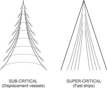
Figure 26
Now we can see why shallow water plays a significant role: fast ferries tend to operate in coastal areas where the depth is limited. Hence they often exceed the critical Froude number, and when travelling at supercritical speed, much of the ship’s power output is concentrated into the leading waves on either side of the diverging wave system [21]. Although relatively small in height, they travel fast, they are persistent, and they pack a considerable punch. With their high energy content they can travel for many kilometres and arrive at a distant location without warning long after the ship has passed, increasing rapidly in height as they approach the shoreline. Without any change in the ship’s velocity, the wave system of a vessel that is travelling several kilometres offshore can change abruptly from ‘sub-critical’ to ‘critical’ if it enters shallower water, and the resulting bow waves can cause damage. An extreme example occurred in 1999, when a man died after being swept from a small fishing boat on the east coast of England in the wake of the Stena HSS Discovery, whose bow wave had risen to a height of 4m as it travelled over a sandbank nearby [10].
Conclusion
According to Thomson’s theory, a ship’s bow makes a beautiful wave pattern as it moves through the water. One is tempted to think of the waves in the ship’s wash as material objects that are carried along by the vessel for the duration of the voyage, but the water itself stays behind: the particles orbit a fixed position, and the circular motions give the impression of crests and troughs moving along with the ship. What does move is the energy that the hull feeds into the water: it flows in the same direction, but more slowly, at half the vessel’s speed. And lagging behind the vessel, it creates new waves continually at the trailing edge of the wash, whose area grows steadily over time. In principle, one imagines, the wave pattern contains historical information about the ship’s progress: how fast it is moving, how long it has been at sea, and how far it has travelled. Thomson’s analysis also explains how a ship’s resistance to motion is related to its speed. The bow and stern wave systems interact, so the resistance increases with increasing speed but not in a smooth manner: uniquely among moving vehicles, the upward trend is interrupted by a series of rises and falls that reflect the changing degree of interaction as the wavelengths increase relative to the length of the hull. This interaction also explains why (other things being equal) a long hull travels faster than a short one.
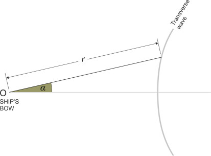
Appendix: Formulae for tracing out the wave crests in the ship’s wave pattern
The layout of the wave crests can be traced using polar coordinates \(r\), \(\alpha\) centred on the ship’s bow as shown in figure 27. Number the transverse wave crests 1, 2, 3, ... in order astern. The locus of the \(n\)th crest [7] is given by:
(18)
\[\begin{multline} r \quad = \quad \left( -\frac{\pi}{4} + 2n\pi \right) \frac{V^{2} \cos^{2} \theta_{1}}{g \cos(\theta_{1}-\alpha)} \\ \text{for } n = 1,\ 2,\ 3\text{...,} \quad 0 \le \alpha \le \arcsin \left( \frac{1}{3} \right) \end{multline}\]where
(19)
\[\begin{equation} \theta_{1} \quad = \quad \frac{1}{2} \alpha - \frac{1}{2}\arcsin(3 \sin \alpha ) \end{equation}\]Figure 27
Likewise the locus of the \(n\)th diverging wave crest [7] is given by
(20)
\[\begin{multline} r \quad = \quad \left( \frac{\pi}{4} + 2n\pi \right) \frac{V^{2} \cos^{2} \theta_{1}}{g \cos(\theta_{2}-\alpha)} \\ \text{for } n = 1,\ 2,\ 3\text{...,} \quad 0 \le \alpha \le \arcsin \left( \frac{1}{3} \right) \end{multline}\]where
(21)
\[\begin{equation} \theta_{2} \quad = \quad \frac{1}{2} \alpha - \frac{\pi}{2} + \frac{1}{2}\arcsin(3 \sin \alpha ) \end{equation}\]Both sets of waves are plotted in figure 13 for a ship moving at 15 knots.
Acknowledgements
Figure 1: Photo by Dadero posted at Wikimedia Commons (public domain) https://commons.wikimedia.org/wiki/File:Bodensee_at_Lindau_-_DS<a href="book?code=C0696">C0696</a>2.JPG (accessed 12 May 2021).
Figure 2: USRA (Universities Space Research Association) Picture of the Day, https://epod.usra.edu/blog/2009/08/boat-wakes-from-above.html (accessed 19 January 2021), photo by kind permission of Prof Lee Anne Willson, Iowa State University, personal web site https://www.physastro.iastate.edu/people/lee-anne-willson, email: lwillson@iastate.edu
Figure 24: NASA photo of supersonic shock waves created by a Northrop T-38 jet trainer, posted at https://www.nasa.gov/centers/armstrong/features/supersonic-shockwave-interaction.html (accessed 19 October 2020).
Figure 26: Boat sailing the Lyse fjord in Norway. Picture taken from the Preikestolen by Edmont, posted at https://upload.wikimedia.org/wikipedia/commons/thumb/5/5c/Fjordn_surface_wave_boat.jpg/420px-Fjordn_surface_wave_boat.jpg, and licensed under the Creative Commons Attribution-Share Alike 3.0 Unported license 23 Jan 2015, accessed 01 June 2016