The fluid continuum

Eventually Newton’s successors developed a new set of principles for analysing fluid flow. It followed a battle of intellectual discovery that drew in many of the world’s great physicists and mathematicians, including the Bernoulli family and their disciples. The first breakthrough took place during the 18th century, when Leonhard Euler (1707-1783), at the time the world’s greatest mathematician, realised how to model the behaviour of a moving fluid. Euler was born in Switzerland and tutored in mathematics at the University of Basle by Johann Bernoulli. He soon became a close family friend [1]. Unlike his contemporaries, Euler visualised the region through which a fluid moved as an array of small boxes or elements, each having a fixed position in three-dimensional space. Assuming the flow was steady over time, he would focus on the fluid that occupied one of the boxes at any particular moment and consider how it interacted with its neighbours, given that frictional forces were negligible. The idea was to produce a system of equations that would yield the fluid velocity and pressure within each of the boxes that made up the flow field. This contrasted with Newtonian mechanics, where scientists were accustomed to tracking the movement of an object along its entire trajectory.

The governing equations

Euler didn’t succeed in predicting fluid motion in any particular situation. What he did do was to build a framework that engineers and physicists still use today for analysing those parts of the flow field where friction can be neglected. The framework is built on two sets of equations. The equations in the first set relate to continuity – the common-sense requirement that matter can’t be created or destroyed within the flow field: what goes into each box must come out. Although they look a lot simpler than the equations in the second set, during the 18th century they were far from easy to solve using the methods available at the time. But they tell us a great deal about the way a fluid moves, and yield a ‘map’ showing the speed and direction of fluid motion at each point. They are the equations on which we’ll concentrate in this Section.

The equations in the second set bring in a further dimension: pressure. They are simultaneous equations that describe the forces acting between the fluid elements, modelled in terms of Newton’s second law applied to each element as if it were a solid body. From this second set one can work out the pressures that arise in the fluid, which you need to know if you are trying to assess the behaviour of a moving vehicle, for example, a racing car. They are non-linear simultaneous partial differential equations in two or three dimensions that no-one in Euler’s day knew how to handle. It was some time before another member of the Bernoulli family was able to extract useful conclusions from them, a topic we’ll postpone until the next Section (F1918).

The continuity equation

The idea of a continuum crops up in many areas of classical physics. It underlies many phenomena such as the flow of heat and electricity, together with less tangible things such as gravitational and magnetic fields that don’t actually move but extend over three-dimensional space. They all obey the same equation insofar as the quantity of ‘stuff’ is conserved in some sense, either from place to place or over time. Here we are concerned with a fluid such as air or water in which there are no gaps or discontinuities. Assuming the motion is steady over time, the rate at which fluid mass enters a particular region of three-dimensional space and the rate at which it leaves must be equal.

Figure 1

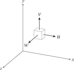
There are different versions of the continuity equation depending on the assumptions made about the fluid and the way it moves. Here we’ll assume an incompressible, frictionless fluid in steady, irrotational flow. If we’re working in three dimensional space, the velocity at any point has three components \(u\), \(v\) and \(w\) respectively parallel to the \(x\), \(y\) and \(z\) axes. Let’s examine the flow into and out of an infinitesimally small rectangular box that is fixed in position with its edges aligned parallel to the axes as shown in figure 1. The dimensions of the box are \(\delta x\), \(\delta y\), and \(\delta z\) measured parallel to their respective axes.

Figure 2

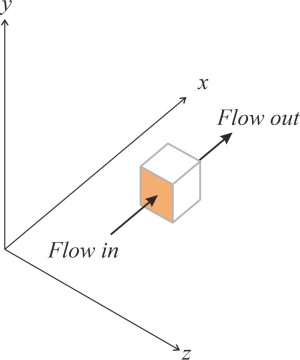
In figure 2 we see the box from a different angle: the face that is highlighted in red has area \(\delta y . \delta z\), and since the fluid is moving through it with velocity \(u\), the volume entering per unit time via that face is \(u \delta y \delta z\). To complete the picture we must calculate the volume leaving per unit time via the opposite face. During the transit of fluid particles through the box, their velocity component in the \(x\) direction will change at some unknown rate \({\partial u}/{\partial x}\). Hence the exit speed at the opposite face is \(u+\left( {\partial u}/{\partial x} \right)\delta x\) and the exit flow is \(\left[ u+\left( {\partial u}/{\partial x} \right) \delta x \right]\delta y \delta z\). One can apply the same reasoning to the other two pairs of faces and combine the results to obtain the following:

and since the total flow out must equal the total flow in, the difference between the right-hand side of equation 1 and the right-hand side of equation 2 must be zero so that

which after cancelling the common factor \(\delta x\delta y\delta z\) leads to Euler’s continuity equation:

In modern textbooks this is usually expressed in vector notation, which is neater and more economical. But we’ll stick to the longhand form here. The question is how to solve this equation for any given set-up where fluid passes around a moving body or along a boundary surface. We want to know what are the values of the velocity components \(u\), \(v\) and \(w\) at any point in the flow field, or some equivalent information that will enable us to build a picture of the fluid motion. The difficulty is that we have three unknowns and only one equation.

The velocity potential

After Euler died, Joseph Lagrange (1736-1813) took up the challenge. Born in Italy, Lagrange had once been Euler’s pupil. His most important work, entitled Mécanique Analytique, was intended to summarise all mechanical science in one publication. It contained a seminal idea. It wasn’t a strategy to solve the Euler equations – at least, not directly. Instead he introduced another variable to replace the velocities \(u\), \(v\) and \(w\): the velocity potential denoted by \(\phi\). The velocity potential is a function that yields the velocity component \(u\) in the \(x\)-direction when differentiated with respect to \(x\). In the same way, it yields the velocity component \(v\) in the \(y\)-direction when differentiated with respect to \(y\), and similarly for \(z\) [4] [5]. Hence:

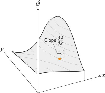
So what is \(\phi\)? In one sense, it is just a function of \(x\), \(y\) and \(z\), a number that has a particular value at each point in the flow field. It’s easier to visualise for two-dimensional flow, because you can picture it as a landscape whose surface rises and falls from place to place as shown in figure 3. The height of the land as such is not important – what matters is the rate at which it changes, in other words the slope. Assuming such a landscape can be constructed, the slope of the ground measured in any particular direction (for example parallel to the \(x\)-axis at the point marked with a red dot) tells you the component of velocity in that direction. If the ground slopes steeply upward, the velocity is large. It’s a clever idea because if it works, the potential replaces three unknown variables with one.

Figure 3

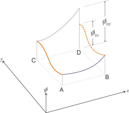
However, it’s not clear whether such a surface can exist: it implies that any variations in the velocities \(u\), \(v\), and \(w\) from place to place within the flow field are somehow related, whereas in real life, the slopes in the \(x\)-direction and those in the \(y\)-direction, for example, might be geometrically incompatible. The problem is highlighted in figure 4, which shows the \(\phi\) ‘landscape’ over a rectangular area within a two-dimensional flow field. The blue curve shows how the potential varies in the \(x\)-direction along the line from A to B, when defined so that its slope in that direction equals the velocity \(u\). The red curve shows how it varies in the \(y\)-direction along the line from A to C when defined so that its slope equals the velocity \(v\). So far, so good – there is no reason why a landscape surface shouldn’t pass through both these lines. Now we want to extend the surface to a fourth point D. There are two paths to D, respectively dotted blue and dotted red, that track the variations in \(\phi\) respectively along CD and BD. The question is whether the values of \(\phi\) predicted by these two curves as they converge on point D actually agree. If they agree, the single surface provides a consistent model for the variations in both velocity fields \(u\) and \(v\), and the velocity potential exists. Otherwise, it doesn’t.

Figure 4

It’s not difficult to determine the conditions under which this will happen, but before doing so, here is an example of a flow field where it most definitely does not. In figure 5, we see water flowing in the \(x\)-direction along the side of a ship’s hull (it could equally well be air flowing over an aircraft wing). The fluid particles closest to the hull stick to the surface, so their velocity when measured relative to the ship is zero. Further away, they travel faster, and for the purpose of this exercise we picture the velocity \(u\) (velocity in the \(x\)-direction) rising linearly with distance \(y\) measured perpendicular to the ship’s side.

Figure 5

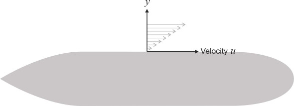
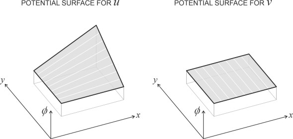
Hence as shown on the left-hand side of figure 6 the potential surface is twisted because the slope in the \(x\)-direction must steepen with increasing \(y\). But what about the slope in the \(y\)-direction? The velocity component \(v\) perpendicular to the ship’s side is everywhere zero, so the velocity potential cannot slope at all in the \(y\)-direction, and on the right-hand side of figure 6 it is shown as a flat plane. Clearly there is a contradiction – the two surfaces are different, or to put it the other way round, no one surface can represent the pattern of variation in both the velocities \(u\) and \(v\). The two requirements are incompatible, and no velocity potential exists.

Figure 6

So what conditions would be required to make the surfaces compatible? It turns out that one condition will do: the flow must be irrotational. It is easy to see that there is a connection between rotation and the existence or otherwise of \(\phi\). In Section F2019 we defined the vorticity as

If the velocity potential \(\phi\) exists, we can substitute for \(u\) and \(v\) via equation 5 and equation 6 to get

The two terms on the right hand side are ‘mixed derivatives’. In each case, the function \(\phi\) is differentiated twice, once with respect to \(x\) and once with respect to \(y\). The only difference is the order in which the two differentiations are carried out, and it turns out that for most practical problems in engineering, the two terms are equal and therefore the vorticity \(\xi\) is zero.
It follows that if the velocity potential exists, the flow must be irrotational, and this is how most textbooks spell out the connection between the two. But it’s not what we are looking for: the fact that all potential flows are irrotational does not prove that an irrotational flow must be potential. A concise demonstration of the latter is set out in [7], but it’s not easy to follow. Let’s return for a moment to figure 4, and track the value of \(\phi\) along the two alternative routes from A to D, adding up small changes in \(\phi\) as we progress. We’ll start at A and denote the initial value by \(\phi_{A}\). Integrating along the route ABD gives a value that we’ll denote by \(\phi_{D1}\), while integrating along the route ACD leads to a value \(\phi_{D2}\). We have:

Subtracting the one from the other gives

The terms on the right-hand side of this equation have a familiar look. Each refers to the tangential velocity along one side of a rectangular area. The first two terms are path integrals of the tangential velocities along the sides AB and BD, measured positive in the anticlockwise direction. The last two terms are likewise integrals of the tangential velocities around the remaining two sides, but they are measured in the clockwise direction. So in the first two terms we can replace the symbols \(dx\) and \(dy\) by the symbol \(ds\) representing distance anti-clockwise around the perimeter, while in the second two terms we’ll replace \(dx\) and \(dy\) by the symbol \(-ds\). Equation 12 then becomes

and a little thought shows that this is equal to the circulation for the area ABCD as defined in equation 1 in Section F2019. If the flow is irrotational, by definition the circulation is zero, which tells us that \(\phi_{D1}\) equals \(\phi_{D2}\). It follows that the potential \(\phi\) gives a valid and consistent representation of the flow velocities, in other words, \(\phi\) exists. In such cases, the flow pattern acquires a special status – it is called a ‘potential flow’, and the contour lines are called ‘equipotentials’.

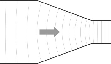
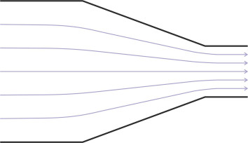
If it exists, the potential surface defines a landscape whose height \(\phi\) at any point in the flow field will tell you a lot about the fluid velocity at that point. Specifically, the slope measured in any given direction tells you the component of fluid velocity in that direction. You can choose any direction you want. For example, you could measure the slope along a contour line. By definition, the height of a contour line is fixed so the slope is zero and the velocity component in that direction must be zero too. But it might be more useful to measure in the direction of the steepest slope, which by definition lies at right-angles to the contour line. A measurement in this direction tells you the resultant velocity. In places where the contours are close together, the slope is steep and the fluid velocity is high. In places where the contours are spaced far apart, the slope is shallow and the fluid velocity is low. Figure 7 is a sketch of the equipotentials for a fluid passing through a constriction in a pipe: the lines get closer together as the pipe gets narrower, indicating a steeper ‘slope’ and hence increased velocity at the constriction.

Figure 7

The stream function

The equipotentials help us to visualise how a fluid behaves in a given situation. But they don’t tell us - at least not directly - the direction in which the particles are actually moving. But one can sketch a second set of lines at right-angles to the equipotentials that do exactly that. They’re called streamlines, and they can be generated by another system of equations that embody a new variable \(\psi\) known as the stream function. Unlike the velocity potential, the stream function applies only to two-dimensional flow. It is defined by

Figure 8

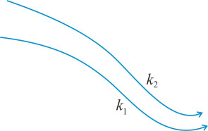
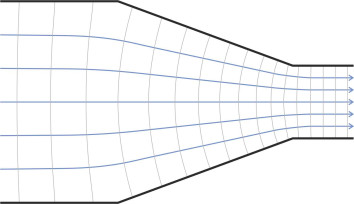
The idea is that along any streamline, \(\psi\) has a constant numerical value, say \(k_{1}\). Such a streamline is pictured in figure 8, along with a neighbouring streamline for which the value of \(\psi\) is \(k_{2}\). The two streamlines act like a pipe or a conduit: fluid can’t cross a streamline so under steady flow conditions the rate of flow is the same everywhere along the conduit. Its magnitude is \(k_{2} - k_{1}\). A complete set of streamlines is sketched in figure 9 for the same flow field as the one shown in figure 7. You can see that the streamlines run closer together as the fluid enters the constriction.

Figure 9

Comparing these two figures, you might guess that the stream function and the velocity potential are closely related because they convey the same information in two different ways. We have already hinted that at any point on an equipotential contour, the direction of flow should lie at right-angles to the contour, and so it proves: one can demonstrate mathematically that the equipotentials and streamlines are everywhere orthogonal. They form what is known as a ‘flow net’ (figure 10). A few decades ago, it was common practice for engineers to estimate the seepage of water through the soil under a dam, for example, by sketching the flow pattern in pencil and adjusting the streamlines and equipotentials by eye until the flow net was made up of roughly square-shaped elements.

Figure 10

The Laplace equation

But we want to plot the curves more precisely using a mathematical formula. So let’s transform the continuity equation into one that we can solve, an equation that contains only one unknown. Substituting \({\partial \phi }/{\partial x}\) for \(u\), \({\partial \phi }/{\partial y}\) for \(v\), and \({\partial \phi }/{\partial z}\) for \(w\) in equation 4 we get

Originally formulated by the French mathematician Pierre-Simon Laplace (1749-1827), this is known as the Laplace equation. In two dimensional flow it reduces to

An equivalent function can also be derived for the stream function. Assuming irrotational flow in two dimensions, we know that the vorticity must be zero, in which case equation 8 simplifies to

If we now substitute equations equation 14 and equation 15 into equation 18 and rearrange the result, we arrive at the Laplace equation once more, this time with \(\psi\) as the unknown:

Let’s remind ourselves that the flow must be inviscid, incompressible and irrotational – in other words, a ‘potential flow’. Then, the Laplace equation will determine the way the fluid moves around a vehicle or though an enclosed space on the basis of very little information other than the shape of the solid surface. We actually have two versions here - equations equation 17 and equation 19 - but they are functionally equivalent and lead to the same conclusions. Using only the continuity of the fluid as the guiding principle, either will enable one to predict the speed and direction of motion at every point within the flow field. Neither the fluid density nor the forces that arise among the particles have any bearing on the outcome. The question is how to solve the equations. Laplace himself developed a method for solving partial differential equations of this kind, and although he never applied it to Euler’s problem directly, it helped others to complete the task. Over the years, the solutions have been research intensively, enabling flow fluids to be modelled over a wide range of situations. Any solution is a potential fluid flow. There are many possibilities, for example:

The problem is to find a solution that can be configured to fit the boundary conditions. In equation 20 the symbols \(p\), \(A\), \(B\), \(C\) and \(D\) are numerical constants whose values can be fixed independently at any level one might desire – whatever values you choose, the solution will still satisfy Laplace’s equation, as you can see if you substitute the right-hand side for \(\phi\) in equation 17 and carry out the differentiation yourself. So the trick is to work out the values that mould the resulting streamline pattern to fit the solid boundaries that occur in your flow field. If you are trying to determine the flow round a moving object, your boundary conditions will echo the shape of the object, setting constraints on the flow pattern so that the streamlines follow its surface profile. This is easy if the boundaries are straight lines, but it becomes more difficult if they are curves. Unfortunately, the body surface of a vehicle such as an automobile can’t be represented as a simple mathematical curve. It’s too lumpy and irregular, and in its raw form, the equation doesn’t help. Instead one can use one of its beautiful properties, namely that it is linear, so you can build up a picture of the flow around a complicated shape by superposing basic flow patterns. Just add together the velocity potentials as will be explained shortly. You might want to look up this method together with more advanced methods in the literature, examples of which are listed under ‘Further reading’ at the end of this Section. More commonly nowadays, the engineer will break down the flow field into small elements and use computer software to analyse the elements one by one using an iterative method that ensures continuity together with dynamic equilibrium in cases where the fluid is viscous. The most advanced techniques have been given the collective label ‘computational fluid dynamics’, and they’ll be reviewed briefly in Section F1817.

Mapping the streamlines

One can demonstrate the underlying principle by working out the flow of air or water round a body of simple geometrical shape. Rather than tinkering with the boundary conditions, we’ll analyse two or three elementary flow fields, none of which actually contain a moving body. Then we’ll add them together to create a boundary of the shape we want – the process is easier to carry out than it is to explain.

Figure 11

Uniform flow field

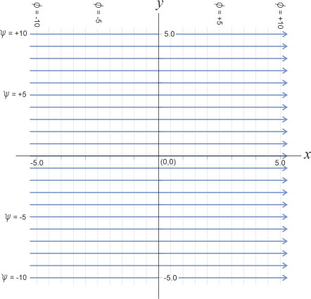
The first elementary flow field is shown in figure 11. It is a two-dimensional field in which the flows are measured in units of area per unit time rather than volume per unit time as would be the case in three-dimensional flow (if we want to think of the flow in a more natural way as the volume per unit time we can imagine the flow field as one unit thick). The blue lines are the streamlines and the grey lines are the equipotentials. The fluid is moving in parallel straight lines from left to right at velocity \(u = V\), and since \(V\) is constant throughout the flow field, equation 5 tells us that

where \(C_1\) is an arbitrary constant. After integration, we get

This means that each equipotential is a straight line parallel to the \(y\)-axis (and you can check that this solution satisfies the equation by substituting for \(\phi\) in equation 16). Suppose the velocity \(V\) is 2 m s\(^{-1}\). For convenience we want to draw the equipotentials at regular increments of 1 m² s\(^{-1}\), and we’ll put \(C_{1} = 0\) so the zero equipotential lies on the \(y\)-axis. Since by definition the rate of change of \(\phi\) per unit distance in the \(x\)-direction is \({\partial \phi }/{\partial x}\), we have

so the equipotentials must be spaced apart a distance equal to the \(\phi\) increment divided by \(V\), or (1 m² s\(^{-1}\))/(2 m s\(^{-1}\)) = 0.5 m. They are shown in grey in figure 11. Now for the streamlines: following a similar line of reasoning we deduce that they are straight lines parallel to the \(x\)-axis:

For convenience we want to draw them with successive \(\psi\)-values set at equal increments of 1 m² s\(^{-1}\), so like the equipotentials they will be spaced apart a distance equal to 0.5 m, and we’ll put \(C_{2} = 0\). The resulting streamlines are shown in blue in figure 11. As you would expect, when plotted together the equipotentials and streamlines form a rectangular grid.

Figure 12

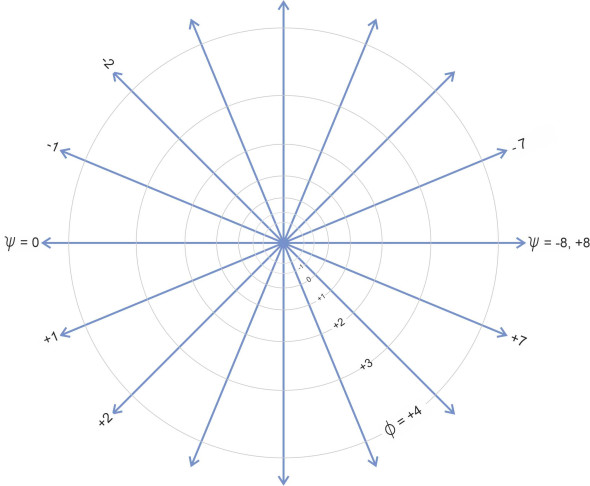
Point source

The flow field in figure 12 is more interesting. It contains a point source, a small hole through which fluid is injected at a constant rate into the flow field and fans out equally in all directions. For this example we’ll switch to circular coordinates (\(r\), \(\theta\)). By convention the angle \(\theta\) is measured anti-clockwise starting at zero on the \(x\)-axis. If the rate of flow \(q\) is measured in units of area per unit time, the fluid disk expands at a rate \(q\) m² s\(^{-1}\), and during a short time interval \(\delta t\) it will create an annulus of area \(q \delta t\). If the radius of the annulus is \(r\) and its width \(\delta r\) as shown in the Figure, its area must be \(2 \pi r \delta r\) so we can write

or in the limit:

The term on the left-hand side is the rate at which the radius increases, which is simply the velocity of the fluid. We know that when the velocity is measured in the \(x\)-direction the velocity potential satisfies equation 5, so if we substitute \(r\) for \(x\) we can interpret equation 5 to mean that

which on integration becomes

where \(C_{3}\) is an arbitrary constant. We can stipulate that \(C_{3}\) is zero at the origin so that when the integrals are evaluated we get

It’s not too difficult to derive an equivalent expression for the stream function. Each streamline is a straight line radiating from the origin at some angle to the x-axis. The total outflow is divided equally around the directions of the compass so that for the streamline at angle \(\theta\),

In figure 12, we have assumed a flow value \(q\) equal to 16 m² s\(^{-1}\) , with both equipotentials and streamlines drawn at intervals of 1 m² s\(^{-1}\). The constant \(C_4\) is set at - 8 m² s\(^{-1}\) so that the streamline corresponding to \(\psi = 0\) lies on the x-axis.

Particles on a circular path

We’ve examined two elementary flow fields in which the particles move in straight lines, so let’s try something more advanced and see what happens when their paths are curved, specifically in a circular orbit. Figure 13 shows a fluid element that is enclosed between two streamlines. The radius of the inner streamline is \(r\) and that of the outer streamline is \(r + \delta r\). We’ll denote the velocity along the inner streamline by \(U\), and that along the outer streamline by \(U + \delta U\).

Figure 13

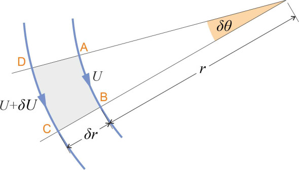
Our goal is to work out how the velocity varies as a function of \(r\), assuming that the flow is irrotational and therefore that the circulation \(\delta \Gamma\) around the fluid element is zero. The derivation is not rigorous but the result will be confirmed via a different route in Section F1818. According to equation (4) in Section F2019, to find the circulation we must integrate the tangential velocity component with respect to distance measured around all four sides of the fluid element, taking the velocity as positive anticlockwise. For sides AD and BC the tangential velocity component is zero. For side AB it is \(-U\) and for side CD it is \(U + \delta U\). Hence

The terms \(-U r \delta \theta\) and \(+Ur \delta \theta\) cancel out; after omitting the term \(\delta U \delta r \delta \theta\) which is negligible compared with the others and rearranging, this becomes

This is equivalent to

which we can integrate to get

One concludes that in a potential flow, the velocity of fluid particles moving along a circular path is inversely proportional to their path radius, or to put it crudely, the particles on the inside of the curve move faster than those on the outside – and close to the centre of the curve, they move a lot faster. This might not appear significant at first, but it’s a fundamental characteristic of fluid behaviour, and it can profoundly affect a moving vehicle. For example, air will accelerate as it curves over the roof of an automobile at speed, or over the top of an aircraft wing. As will become clear in the next Section, in both cases the acceleration leads to a reduction in pressure and an upward force. Equation 33 also goes some way towards explaining the pattern of motion in a free vortex, a matter to which we’ll return in more detail later in Section F1818. In theory, the velocity increases without limit close to the central axis.

Towards a streamlined vehicle

The fact that the equation is linear allows us to superpose two flow fields simply by adding their velocity potentials together. So let’s try this with the uniform flow field and the point source flow field, whose velocity potentials are embodied respectively in equations equation 22 and equation 29. Note that equation 22 is expressed in Cartesian coordinates while equation 29 is in polar coordinates. In what follows, polar coordinates are easier to use so we’ll convert the uniform flow field equation accordingly to give

Then adding this component to the point source component in equation 29 we get

and noting that \(C_{1} = C_2 = 0\), after re-arrangement this becomes

Figure 14

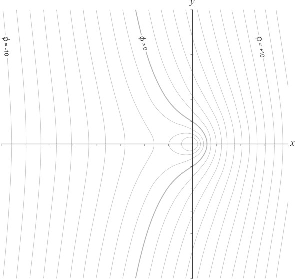
When set up on a spreadsheet, this formula can be evaluated for different values of \(\phi\) to generate the set of equipotential curves shown in figure 14. A similar process yields an equation for the streamlines:

which, on setting \(C_{3} = 0\) and \(C_{4} = -8\) yields the streamline pattern that is shown together with the equipotentials in figure 15.

Figure 15

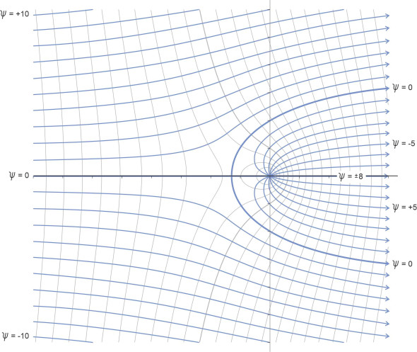
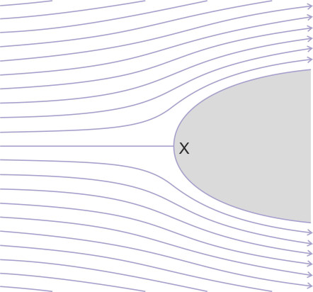
The pattern of streamlines shows how the two flow fields interact when they are superposed. As you might expect, particles in the uniform flow approaching from the left deflect the motion of those emerging from the point source, pushing them across to the right. But does this tell us anything useful? figure 15 reveals an interesting possibility. By definition a streamline is a curve that no particle can cross, so in frictionless flow, any particular streamline can be interpreted as a boundary surface. The most striking example is the streamline \(\psi = 0\). Figure 16 depicts the area to the right of this streamline as the front of a solid object that deflects the flow around either side. In effect, we have modelled the nose of a streamlined vehicle, the ‘Rankine nose’ so named after physicist Lord Rankine who worked in this field during the 19th century. The pattern is quite close to what happens near the front of a vehicle in real life, even for moderately viscous fluids. You can see that the flow is sluggish around the nose, and in fact there is a stagnation point at the point labelled ‘X’ where the fluid velocity is zero. What happens at the rear is a different matter that we’ll leave aside for now.

Figure 16

Circular cylinder

We’ve ‘created’ the flow pattern round the nose of a streamlined vehicle from two elementary flow fields, the uniform flow field and the point source. One can combine other flow fields in a similar way. Each combination generates a flow pattern that can be interpreted as the fluid motion round a body having a simple geometrical shape, and there are many examples to be found in fluid mechanics textbooks. An instructive case arises when a source and sink are combined together with a uniform flow field to simulate the flow round a cylinder immersed at right-angles to the direction of flow as shown in figure 17. The fluid diverges around either side before converging again downstream; the downstream pattern is a mirror image of the flow upstream. Notice that because the fluid is non-viscous, it encounters no friction as it slides over the cylinder surface, but its speed still varies considerably from place to place within the flow field.

Figure 17

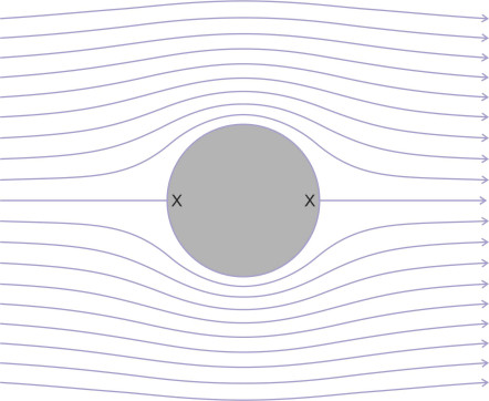
In principle, for a body of simple geometrical shape one can calculate the fluid velocity at each point around the body surface and indeed at any point within the flow field. We’ll just quote the result set out in [6], again using circular coordinates. If the point in question subtends an angle \(\theta\) at the origin (measured anti-clockwise starting from zero on the \(x\)-axis), the tangential velocity \(u_{\theta s}\) at the circular surface is given by:

As you might expect, the fluid moves more slowly at the front and rear than in the undisturbed stream, but faster around the flanks on either side. To be precise, it is zero at each of the stagnation points, but twice the undisturbed stream velocity at \(\theta = \pi /2\) and \(\theta = 3 \pi /2\). We’ll need this result in the next Section.

More on frictionless flow

We’ve plotted the flow pattern showing how an ideal fluid moves around a ‘Rankine nose’ and how it moves around a circular cylinder, two simple geometrical shapes. Before moving on, let’s examine a couple of questions that turn out to be important later.

What the pictures don’t tell us

Plotting the streamlines and equipotentials enables one to visualise the motions of fluid particles as they pass around a moving vehicle. It’s particularly useful to know how their velocities vary from place to place, because as we’ll see in the next Section, it’s the local velocity that determines the pressure exerted on the body surface. But the plots don’t actually show the velocities, at least not directly. We know they rise and fall with the spacing between adjacent streamlines, but their precise values remain hidden from view. We can’t track the whereabouts of individual particles over time and compare their progress against that of their neighbours. The plot of the equipotentials in figure 15 gives the impression that the fluid particles are like soldiers marching in formation along a parade ground, diverging around an obstacle and re-forming in line abreast downstream before departing from the right hand side of the diagram. The question is important if one is trying to understand the behaviour of an aircraft wing – it is tempting to imagine that when two neighbouring air particles diverge at the leading edge, one passing over the top and one passing underneath, they arrive simultaneously at the trailing edge, and that since the upper route is slightly longer, the air travelling over the top must travel slightly faster. On occasions in the past, this idea has been used to explain the phenomenon of ‘lift’.

In reality that’s not what happens. Let’s return to figure 17. Please ignore the fact that the cylinder is symmetrical about the \(x\)-axis and therefore can’t generate any lift – we are only going to look at the top half of the flow field. If we label the particles entering the left hand side of the diagram at a particular moment, and track their motion across it, they won’t all arrive at the right-hand side at the same time. The cylinder obstructs the flow. In particular, it retards the motion of particles passing close to its surface relative to those some distance away where the cylinder has less influence on the flow pattern. The nearby particles take longer to reach the right hand side of the flow field, and in fact a particle arriving along the \(x\)-axis (where \(\theta = 0\)) never gets there at all, becoming permanently lodged at the first stagnation point.

A question of scaling

Our second issue concerns scaling, and it leads to a more positive conclusion. Each of the flow nets described in this Section is calculated on the basis of an assumed value for the undisturbed stream velocity \(V\). If we are modelling a vehicle moving through a stationary fluid, \(V\) represents the velocity of the vehicle, and in the case of the Rankine nose, \(V\) was fixed at 2 m s\(^{-1}\). But what would happen if the vehicle were to speed up or slow down? A little thought shows that the velocities of the fluid particles would change by the same factor \(k\) throughout the flow field. Why? Because the geometry is unaffected. If the vehicle velocity increases by a factor \(k\), we can simply increase the value of \(\phi\) associated with each equipotential in figure 14 by the same factor, re-label it accordingly, and leave it in position. Similarly with the streamlines: we change the value of \(\psi\) associated with each streamline in figure 15 to \(k \psi\) and leave its shape unchanged. Then all the velocities rise by a factor \(k\). This is a fundamental property of ideal fluid flow: the particle velocities scale up and down but the geometry doesn’t change. Under specified conditions, this means that one can describe a potential flow pattern in purely geometrical terms, and we’ll use it to advantage in Section F1918 to deduce a scaling law for fluid forces.

High-speed flow

However, the geometry does change when the velocity rises above a certain threshold. Up to now, we have assumed that the fluid is incompressible, whereas a fast-moving aircraft will cause the air to contract and expand as it passes over the wings and fuselage. As the aircraft approaches the speed of sound, the air particles form a shock wave as described earlier in Section F2019. The supersonic ‘bang’ that you hear when an aircraft passes through the sound barrier is the same kind of noise as the one made by a shell or a bullet fired from a gun. People have known for a long time that bullets travel faster than the speed of sound, but it wasn’t until 1887 that the physicist and philosopher Ernst Mach first observed shock waves in the laboratory and published his results [2]. Today we denote the velocity of a fast-moving vehicle in terms of the Mach number \(M\), which is simply the ratio of the vehicle speed divided by the speed of sound under the prevailing conditions.

Supersonic flow is very different from potential flow, and over the years, researchers have built a distinct theory to help them understand what happens when the velocity of the air moving over the vehicle body surface exceeds Mach 1. In mathematical terms, since the density is no longer constant there is an additional unknown, and another equation is needed to supplement the continuity and momentum equations mentioned so far. This is the ‘equation of state’; it describes how the volume (and therefore density) of an ideal gas changes with pressure. You may have come across it during physics at school, in the form

where \(p\) stands for pressure, \(v\) is the specific volume (volume of air per unit mass), \(T\) is the temperature in degrees Kelvin, and \(R\) is a constant. The specific volume is just the inverse of density, so we can re-write the equation as

which tells us how the density changes with pressure. But you can see the snag: the temperature \(T\) itself is unknown, so we need yet another equation [3] [8], this time an ‘internal energy equation’ that specifies the temperature change associated with any expansion or contraction in the fluid. We are now getting into the realm of thermodynamics – which is not too surprising if you recall that in high-speed supersonic flight, the nose cone of a vehicle can get hotter than the melting point of steel. There are now essentially four equations with four unknowns, and to keep the problem manageable, it is usual to assume that no heat is transferred between the fluid and its environment and that there are no friction losses. In technical parlance, the process is adiabatic and reversible so the entropy doesn’t change. However, the mathematical challenge rises to a new level, and in this web site we won’t go into the details although we can still tackle simple problems and learn something about the geometrical wing shapes and body shapes that are specially suited to high-speed flight.

Where next?

You’ll recall that Euler proposed two sets of equations, and so far, we have studied only the first set, the continuity equations. Assuming an ideal fluid in steady, irrotational motion, these are the equations that determine the pattern of flow around a moving vehicle. The next task is to work out the pressure that the fluid stream exerts at different points on the body surface. To do this, we need Euler’s second set of equations, which bring into play the forces at work within the fluid, and it’s these forces that we’ll examine in the next Section.