
F.1616
Fluid flow and body shape
If there’s a car showroom in your neighbourhood and people are gathered outside, they’re probably staring at a sports car with its body panels glistening under the spotlights. There’s something about a streamlined vehicle that compels one to stop and look. An aircraft can have a similar effect. I once arrived at a provincial airport to join an overseas flight. The passengers had to walk under the wing to board the plane, and I paused to admire its shape from close quarters: the engine nacelles, the undercarriage, and the fuselage overhead. From below, they weren’t shiny nor even particularly smooth, but somehow blank and purposeful as if the whole contraption had just arrived from an alien world. In a sense it had. A jet airliner is a pressurised capsule, designed to hold passengers in a semi-vacuum ten kilometres above the earth’s surface while flying at nearly the speed of sound.
Passenger jets are a relatively recent development, but streamlined shapes are not: centuries ago, the craftsmen who built wooden ships knew that a smoothly curved hull would glide along the water surface more easily than a rectangular box, and with little scientific guidance, they built vessels whose lines we still admire today. The same wasn’t true for vehicles that moved on dry land. Horse-drawn coaches didn’t generate much air resistance, and they were built more like houses on wheels. But eventually, the arrival of mechanical power made aerodynamic performance more important, and engineers began to ask themselves what an automobile should look like. It wasn’t a straightforward task, and it took many decades of research using wind tunnels and road tests to reveal what we now know to be the optimum shape. However, it wasn’t really suited to carrying people or goods on land, and designers turned to other forms instead. To see how they evolved, we’ll review a range of basic shapes and try to draw out the features that make for an aerodynamically efficient vehicle.
Simple shapes
Different vehicles have different shapes. With a little imagination, they can be divided into three broad categories:
- bluff bodies (which may be boxy with sharp corners like a heavy truck, or more complex, with rounded corners and indentations like a saloon car);
- flat sheets like an aircraft wing, and
- slender tubes, like a railway train.
We can summarise the aerodynamic behaviour of a vehicle in any of these categories by looking at its drag coefficient and seeing how it varies with the speed of the vehicle and the nature of the fluid through which it travels.
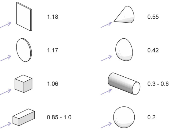
Figure 1
Bluff bodies
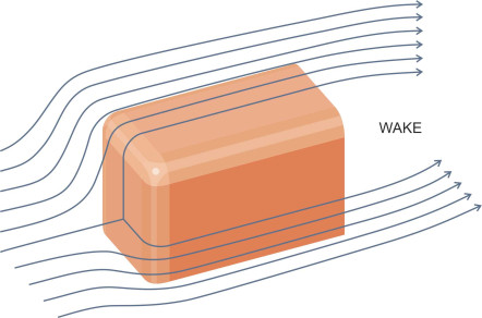
Bluff bodies are typically short and squat. Let’s start with some simple examples, eight of which are listed in table 1 together with their drag coefficients in near-turbulent flow. The shapes themselves are shown in figure 1. The first is a flat plate aligned at right-angles to the flow. The front surface of the plate acts as a barrier, forcing the oncoming fluid particles to turn aside and accelerate outwards along the plate surface as shown in the upper part of figure 2. Each particle gathers momentum that carries it past the edge so it breaks away along a shear layer aligned at right-angles to the flow. The shear layers around the perimeter define the boundary of a wake that forms behind the plate, whose cross-sectional area is greater than that of the plate itself. This implies a high drag coefficient, because the larger the wake the greater the total suction force at the rear that holds the body back. In table 1 you’ll see that the square plate and the circular disc have similar \(C_D\) values: 1.18 and 1.17 respectively.
Figure 2
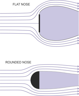
Next comes the cube, aligned with its forward face at right-angles to the flow. Like the flat plate, the forward face causes separation together with a substantial wake: the drag coefficient is a little over 1. But if we replace the flat front with a rounded one, the drag level can fall dramatically, as demonstrated by the hemisphere that appears on the right-hand side of figure 1. The curved surface has two effects. First, it reduces the area of high pressure acting on the nose, and secondly, it postpones separation of the boundary layer until it reaches the flat face at the rear; the line of separation encloses a narrower wake as shown in the lower part of figure 2. In combination with the reduced pressure at the front, the smaller wake exerts less resistance, and the drag coefficient falls to 0.42.
Before moving on, let’s briefly return to the cube and see what happens if we stretch it in the direction of flow so its shape becomes more like that of a lorry or a railway truck. The shear layer bends rearwards, and with a sufficiently long body, it will rejoin the body surface before reaching the rear corner. This limits the diameter of the wake, and as a result, the drag coefficient falls. However, if we continue to lengthen the body, eventually it will rise again because of the viscous friction that develops along the body sides.
| Body | Drag coefficient\(C_D\) | Reynolds number Re | Source |
| Flat plate (square) perpendicular to flow | 1.18 | \(> 10^4\) | [21] |
| Circular disc perpendicular to flow | 1.17 | \(> 10^4\) | [12] [16] [21] |
| Cube aligned with front and rear faces perpendicular to flow | 1.06 | \(> 10^4\) | [19] [21] |
| Rectangular block with smallest faces perpendicular to flow | 0.85 – 1.0 | Unspecified | [4] [9] |
| Cone with half-angle 30\(^{\circ}\), apex first | 0.55 | \(> 10^4\) | [19] [21] |
| Solid hemisphere, curved surface to front | 0.42 | \(> 10^4\) | [13] [19] |
| Cylinder with axis perpendicular to flow | 0.3 – 0.6 | Various | [1] [11] [20] |
| Sphere | 0.2 | \(2 \times 10^5\) | [21] |
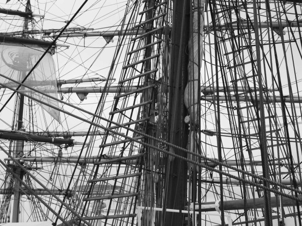
The next body in the Table is a circular cylinder with its axis perpendicular to the oncoming flow. Here, the cylinder is not meant to represent a three-dimensional body like a cube or a cone, but rather a bar of infinite length, and the drag coefficient refers to a unit length not the whole bar. It is relevant because in the world of transport, moving vehicles often have running gear that presents a roughly cylindrical profile to the oncoming flow. The running gear includes axles and suspension struts on high-speed racing cars together with the ropes and cables found on ships and sailing craft (figure 3). All produce significant drag. Early aircraft were braced with steel wires, so thin that one wouldn’t expect them to interfere with the air flow, whereas in reality the resistance generated by a cylindrical wire is the equivalent of a streamlined cross-section around ten times thicker [18]. However, there is a complication. The fluid flow around a cylinder breaks away from the curved surface at two points: as explained previously in Section F1917, at low speeds they are located on the upstream side but move aft at higher speeds. Hence the drag coefficient is sensitive to the Reynolds number. For Re greater than \(3 \times 10^5\) the boundary layer becomes turbulent, separation is postponed, and \(C_D\) falls from 1.2 to somewhere in the region 0.3 to 0.6 depending on the Reynolds number. This is typical of bluff bodies with curved surfaces such as cylinders and spheres: the drag coefficient is not constant, but tends to fall as the Reynolds number increases. By contrast, for boxy shapes, the line of separation that defines the perimeter of the wake tends to remain fixed in place at the sharp corners, and the drag coefficient remains roughly constant.
Figure 3
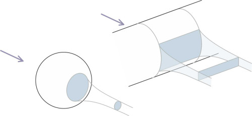
The last ‘bluff body’ considered here is the sphere, the simplest of all geometrical shapes. As you might expect, the drag coefficient falls appreciably as the line of separation moves aft, from a value of 0.5 in laminar flow to 0.2 in turbulent flow. These values are smaller than the corresponding ones for a circular cylinder: it’s because the sphere is a three-dimensional ‘body of revolution’ about an axis aligned parallel to the flow, which effectively reduces the cross-sectional area of the wake as shown in figure 4. In addition, compared with other geometric forms the sphere has the least possible surface area in relation to its volume, and therefore generates low frictional drag. In practice, this is offset by form drag generated within the wake, but nevertheless, as we’ll see later, the sphere’s rounded profile hints at the optimal ‘streamlined’ shape.
Figure 4
Flat sheets and rods
You will often see devices attached to a vehicle that are essentially two-dimensional, flat surfaces aligned parallel to the vehicle axis whose purpose is to extract aerodynamic forces from the surrounding fluid flow. They include (i) a ship’s sails, (ii) the wings that support an aircraft or a marine hydrofoil, and (iii) various kinds of control surface such as a ship’s rudder. In addition, there are other flattened shapes that form part of the vehicle structure but have no hydrodynamic purpose, struts whose cross-section is elongated to minimise drag. As you can imagine, thin, flat shapes of this kind cut through a fluid with very little separation and almost no wake. At subsonic speeds, a wing, for example, has a relatively small drag coefficient, typically of the order of 0.05.
Figure 5
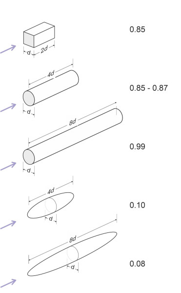
Taking this a step further, you can imagine a one-dimensional body, a thin rod aligned parallel to the direction of flow. Table 2 lists several elongated shapes together with their drag coefficients in turbulent or near-turbulent flow. They are illustrated in figure 5. The drag coefficients vary according to the shape of the nose, the cross-section, and the overall proportions. Let’s examine the rectangular box first. Assuming an approximately square cross-section with the major axis aligned parallel to the flow, it has a drag coefficient roughly equal to 1.0, slightly less than for a cube of the same cross-section. It tends to decrease slightly with increasing length and then increase again, because a significant proportion of the drag for a long, slender body arises from skin friction acting along the top, bottom and sides. If you double its length, you’ll have twice the surface area in contact with the fluid, and common sense suggests that it will produce twice the friction, although in practice things don’t quite work out that way because the dynamics of the boundary layer change as the fluid particles progress from nose to tail along the body surface.
The next two examples shown in figure 5 are cylinders aligned with their axes parallel to the flow. As you might expect, the drag coefficient for a cylinder moving in this way depends partly on its length, because the skin friction increases with increasing surface area. Also, the cylinders shown in the Figure have a flat face at each end, and you’ll have noticed that for all the bodies having flat faces at the front and rear that we have looked at so far, the drag coefficient is relatively high. But this changes if we round off the nose or add a cone at the front: either will reduce the area of high pressure at the front and delay separation at the sides, thereby reducing the overall drag. So let’s go a step further and curve the whole body surface. Our final variant in figure 5 is an ellipsoid, in essence an elongated version of the sphere. Effectively, we’ve tapered the rear as well as the front, so that the cross-section of the body at the point of separation is smaller than its cross-section at the widest point. As the point of separation moves closer to the tail, the the wake narrows and the drag falls. In turbulent flow, the drag coefficient for a sphere is around 0.2. It falls to 0.1 if we stretch the sphere to form an ellipsoid whose length is 4 times the diameter, and to 0.08 if we stretch it further until the length-to-diameter ratio reaches 8:1. We are now approaching an ‘ideal’ form with a very low drag coefficient.
| Body | Drag coefficient \(C_D\) | Reynolds number Re | Source |
| Rectangular box with larger faces aligned parallel to flow, ratio of length-to-breadth 2:1 | \(\sim 0.85\) | Not specified | [9] |
| Cylinder, axis parallel to flow, ratio of length-to-diameter 4:1 | \(0.85 - 0.87\) | \(> 10^4\) | [19] [21] |
| Cylinder axis parallel to flow, ratio of length-to-diameter \(8:1\) | \(0.99\) | \(> 10^4\) | [21] |
| Ellipsoid, ratio of length-to-diameter \(4:1\) | \(0.1\) | \(2 \times 10^5\) | [21] |
| Ellipsoid, ratio of length-to-diameter \(8:1\) | \(0.08\) | \(2 \times 10^5\) | [21] |
The zeppelin
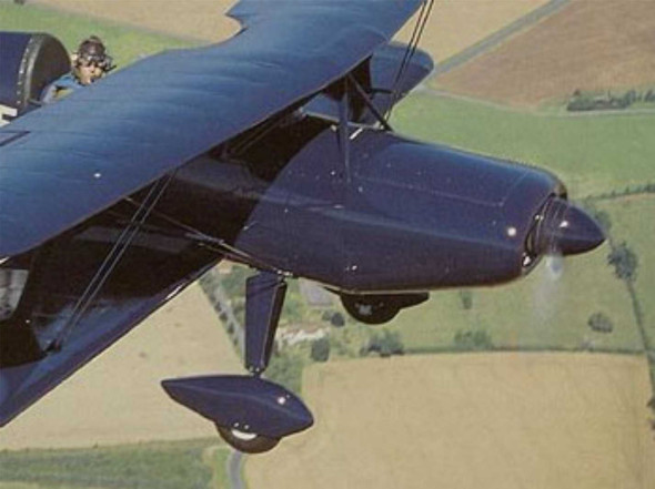
It’s often said that the ideal aerodynamic shape is a teardrop with a rounded nose and pointed tail as shown in figure 6. The name ‘teardrop’ isn’t really appropriate because when it falls through the air, a teardrop doesn’t have a tail and its drag coefficient is quite high. The shape that people have in mind is more like an airship so we’ll call it a zeppelin, after the man who pioneered airship construction during the early 1900s, Count Ferdinand Graf von Zeppelin. He wasn’t the first person to recognise the ‘teardrop’ as an efficient profile. The idea emerged around 1780, when the French hydraulics engineer Pierre-Louis-Georges du Buat (1734-1809) discovered that the rear of a body moving through a fluid had as much influence on the resistance as the front [6]. Around 1809, Sir George Cayley, who built flying models and foresaw the shape of the modern aircraft, deduced the advantage of the rounded nose from the shapes of animals moving through fluids, and like du Buat, understood the importance of a pointed tail. Eventually it was the wind tunnel tests of Fuhrinam and Prandtl during the early twentieth century that confirmed the zeppelin as a shape of minimal resistance [8]. It explains why the ‘spats’ that cover the wheels of many light aircraft have a characteristic zeppelin profile (figure 7), and why racing cyclists wear helmets of a similar shape.
Figure 6
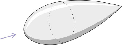
Figure 7
You might wonder about the round nose – at first it doesn’t make sense. If you want to pierce a hole in a piece of wood, you will use a tool with a sharp point. But piercing a fluid is different - neither air nor water resists penetration in the same way as a solid because the particles have no tensile strength: they don’t cling to each other and you don’t need to cleave them apart – at least not unless the vehicle is moving close to the speed of sound. In reality, a rounded nose has less surface area than a pointed one of the same volume, so it produces less frictional resistance. Moreover, a rounded nose is lighter and more compact (which makes a vehicle easier to manoeuvre in a confined space, and less vulnerable to damage).
For moderately large Reynold numbers, the optimum length-to-diameter ratio for the zeppelin is about 2.5 to 1, which yields a drag coefficient widely quoted in the textbooks of around 0.04 [16]. But it’s not a fixed quantity; it falls gradually with increasing Reynolds number for a body moving at high subsonic speeds.
Streamlining
The zeppelin is often described as the most streamlined of all body shapes. It has three distinguishing features: a rounded nose, a pointed tail, and smoothly rounded curves in between. It’s not a new idea. As long ago as the fourteenth century, the hull of a cargo ship below the waterline followed more-or-less the same pattern, inspired by observation of the natural world. Marine architects took their lead from birds and fish, and conceived the plan form shown in figure 8, with the widest beam located a little forward of midships like the body of a mackerel [5] [7]. If it was good enough for a fish, it was good enough for the Navy.
Figure 8
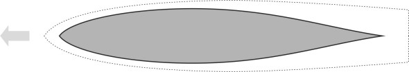
Figure 9
Evolution of the concept
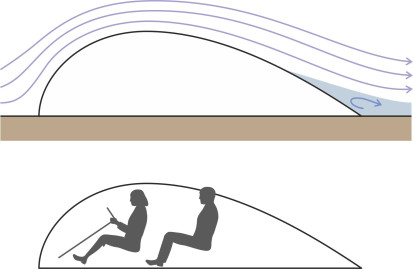
Later during the mid-1800s, steam engines and internal combustion engines appeared, and the rapid pace of development promised much faster vehicles by the end of the century. Scientists began to take an interest in the matter: what would a vehicle of the future look like? On theoretical grounds, pioneers such as du Buat, Cayley and Eiffel envisaged the zeppelin as the perfect shape not only for flying machines, but for land vehicles as well (figure 9). However, an automobile shaped like a zeppelin is not aerodynamically ideal because the air flowing underneath is squeezed between its rounded under-belly and the road surface, which disturbs the flow pattern and raises the drag. A half-zeppelin is a better proposition. Imagine a whole zeppelin in level flight a hundred metres above the ground, say, and slice it horizontally through its centreline. You now have two identical half-zeppelins each surrounded by half the original flow field, the lower one forming a mirror image of the upper one. Now remove everything below the plane of symmetry. As shown in figure 10, we are left with a streamlined body whose length-to-height ratio has increased, being twice the original value at around 5.0. It is skimming along a flat plane which we can visualise as the road underneath, whose surface is moving aft at the same speed as the flow field. The geometry of the streamlines hasn’t changed, so you’d guess that the drag is half the original value. And since the frontal area of the half-zeppelin is also half the original value, the drag coefficient, which by definition equals the drag divided by the frontal area, should remain unchanged at 0.04.
Figure 10
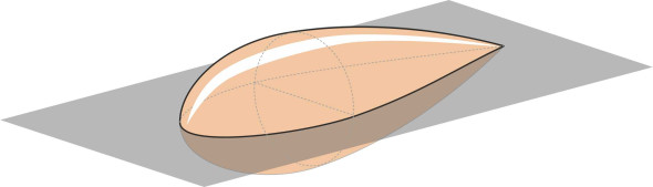
Figure 11
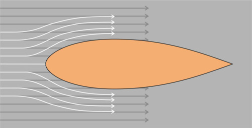
But it doesn’t – for a land vehicle the drag is higher than our theoretical model might suggest. The reason seems to be that the fluid mass and the road surface beneath it are not moving aft in the same direction (figure 11). The fluid particles arriving on the vehicle centreline will divide and accelerate around the sides. In the process, they move diagonally across the road surface at an enhanced speed, and therefore undergo friction on a surface that was not present before the body was sliced in two. The energy loss is manifested in the drag coefficient, which rises from 0.04 to 0.09, and the problem doesn’t end there. To build a practical vehicle, one must add wheels and raise the body a little to provide a suitable ground clearance. The fluid flow inside the wheel arches and beneath the floor is turbulent and generates friction, which in turn adds to the drag and raises the value of the theoretical minimum drag coefficient for a road vehicle to about 0.15 [15].
For flying machines, things are more straightforward. An aerodynamicist will visualise an aircraft as an assembly of parts – for example, fuselage, wings and engine nacelles – each having an independent aerodynamic identity, but joined together and moving at the same speed. One can then shape the parts individually using the zeppelin profile as a standard ‘template’. Even the wings follow the zeppelin profile approximately, at least in cross-section. In principle this should result in an overall drag coefficient of 0.03 or thereabouts, falling to about half that value as the velocity approaches the speed of sound. Although in practice it comes out somewhat higher owing to aerodynamic interference between the parts where they are joined together, the result is better than it might have been with a less efficient template.
Logically, therefore, you’d expect most vehicles today to look like zeppelins. But no! On the ground, you’ll see nothing that resembles a half-zeppelin: our cars are too short and they lack an aerodynamic tail. Railway trains are too long, and they have no tails either – although some have protruding noses. Ships are a little closer to the half-zeppelin model if you ignore the knife-like bow. Passenger jets have rounded noses and pointed tails, but in every case the fuselage is longer and narrower than the zeppelin profile as visualised a hundred years ago. What is going on?
Constraints on the modern vehicle
There are perhaps two reasons why zeppelin-shaped vehicles aren’t very common today. The first is that regardless of its low drag coefficient, the zeppelin doesn’t necessarily produce the least drag in relation to its size, a matter that we’ll take up shortly. The second is that vehicles must satisfy practical constraints that rule out the zeppelin shape. For example, a truck mustn’t project outside a standard traffic lane, which means that in Europe, for example, the width of a road vehicle can’t normally exceed 2.6 metres. The only way you can increase its capacity is to stretch (and articulate) the chassis: it will be longer than a zeppelin, with straight sides. Similarly, a railway train has to fit within a limited width. Typically in Europe, coaches are 3 m wide and 4 m high [10], and coupled in a formation around 200 m long, a passenger train resembles a very long, slender rod with a length-to-diameter ratio of over 50, unequalled by any other kind of vehicle. This implies a large surface area in comparison with other vehicles, so we would expect a railway train to have a high drag coefficient even if it is carefully streamlined. Almost the opposite applies to automobiles, which are short and squat by comparison. But as you’ll see in Section C1416, the zeppelin shape doesn’t work particularly well for cars either, because a zeppelin that is short enough to fit into a regular parking space can’t easily accommodate four seated adults.
The constraints for sea-going vessels are more complicated. A displacement vessel moves at the interface between two fluids, and the complex nature of the marine environment and the conflicting demands made on surface vessels means that no one shape can be optimal under all weather conditions, although there have been certain developments below the waterline such as the bulbous bow that can be justified on scientific grounds. At the same time, there are restrictions on the ship’s cross-section in order for it to pass through major waterways such as the Panama Canal. To maximise the capacity of a hull, this effectively determines the underwater cross-section as a rectangle not much more than 32 m wide with a vertical draft of not much more than 12 m, although new locks have recently been installed to accommodate ships with a beam of 51.15 m and a draft of 15.2 m. And all ships must berth from time to time at a wharf or quayside, which is easier if the sides are straight and parallel in plan.
Practical streamlining
For land vehicles and ships therefore, streamlining involves a compromise. It makes sense to begin with a rectangular box that will conveniently accommodate passengers and cargo, and modify the contours. Let’s take the various parts of the body in sequence, starting with the nose, then the sides, and finally the tail. A boxy profile will induce locally high velocities and cause the boundary layer to separate at the sharp edges, leading to a large wake and considerable drag (figure 12). By comparison, a rounded nose will permit the fluid particles to accelerate more smoothly around the vehicle sides and over the roof. Even with a box-shaped front, one can delay separation by rounding the corners a little as shown in figure 13, which will reduce the drag coefficient by a worthwhile amount [3].
Figure 12
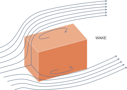
Figure 13
However, none of these alternatives work for supersonic aircraft, which need a pointed nose together with sharp leading edges on their wings: a rounded leading edge is a liability because the shock wave wraps itself around the curve, and the sudden transition from low pressure to high pressure between the shock wave and the body surface accounts for most of the drag. By contrast, a sharp edge presents a relatively small area to the oncoming flow over which the high pressure can act. A ship’s bow cuts the water like a knife too, but it’s there for a different reason, not to reduce the resistance, but to reduce the potentially damaging impact of any oncoming waves. The wave impacts are most severe at the water surface and diminish with depth, so the knife edge can flare into a rounded nose lower down: it is quite common for a ship to have a ‘bulbous bow’ hidden under the water surface that reduces drag by a few percent.
Figure 14
The mid-section of a vehicle body is less important than the nose or tail. The aim is to avoid any discontinuity that might cause turbulence, trigger separation, or generate a vortex, so the engineer will specify a hydrodynamically ‘clean’ surface with the fewest possible excrescences, sharp corners and indentations. What about about further aft? For all vehicle types, we know that a pointed tail can delay separation almost until the apex and thereby minimise form drag (figure 14). A long tail isn’t possible for land vehicles, but a degree of taper towards the rear will at least reduce the diameter of the wake and the area over which the low pressure can act.
How well does it work?
In this web site we are dealing with four main categories of vehicle: ships, railway trains, road vehicles and aircraft. To overcome fluid forces, a vehicle must be supplied with fuel energy, which (a) is expensive, (b) may contribute to climate change, and (c) may create other forms of pollution. So it’s interesting to compare different categories of vehicle in terms of their aerodynamic or hydrodynamic efficiency. This is not a straightforward exercise because among the vehicles in any one category there are wide variations in resistance according to the age of the vehicle, its size, and its cruising speed. Furthermore, there are different ways of measuring aerodynamic efficiency. So we’ll choose – somewhat arbitrarily – a single example from each category, work out its drag coefficient, and see where this leads.
Results for different vehicle types
We’ll start with ships. When crossing the ocean, a ship will experience two forms of resistance that are common to all vehicles: form drag and friction drag. The friction drag is sensitive to the smoothness of the hull, and particularly the degree of fouling by marine organisms. On top of form drag and friction drag, it will experience resistance caused by (a) the rise and fall of the hull together with the impact of waves on the bow, and (b) independently of weather conditions, the waves that the hull itself creates, which draw off energy. For all these reasons, marine architects don’t recognise the drag coefficient as a meaningful indicator of the total resistance, but nevertheless we’ll estimate its value for a well-known class of cargo vessel, bearing in mind that the result doesn’t reflect the wide variations that can occur under different operating conditions at sea. The vessel we’ll choose is the standard M4 bulk carrier. Applying a regression model that predicts approximate drag values based on the ship’s dimensions [22], we estimate a total drag at about 906 kN at a cruising speed of 7.72 ms\(^{-1}\) (15 knots). When we substitute this value for \(D\) in the classical drag formula (see equation 1 below), together with the cruising speed and lateral cross-sectional area of the wetted hull, this implies a drag coefficient of about 0.081. The details are set out in the third column of table 3.
| Vehicle category | M4 bulk cargo ship | ETR 500 passenger train | Medium family car | Boeing 747 passenger jet |
|---|---|---|---|---|
| Fluid density \(\rho\) (kg m\(^{-3}\)) | \(1025\) | \(1.226\) | \(1.226\) | \(0.4135\) |
| Dynamic viscosity \(\mu\) (N s m\(^{-2}\)) | \(1.08 \times 10^{-3}\) | \(1.79 \times 10^{-5}\) | \(1.79 \times 10^{-5}\) | \(1.46 \times 10^{-5}\) |
| Length \(L\) (m) | \(243\) | \(250\) | \(4.67\) | \(71.0\) |
| Cruising speed \(V\)(m s\(^{-1}\)) | \(7.72\) | \(83.3\) | \(33.3\) | \(250\) |
| Reynolds no Re | \(1.78 \times 10^9\) | \(1.43 \times 10^9\) | \(1.07 \times 10^7\) | \(5.03 \times 10^8\) |
| Frontal area \(A\)(m2) | \(366\) | \(9.78\) | \(2.13\) | \(180\) |
| Drag \(D\) (kN) | \(906\) | \(64.5\) | \(0.406\) | \(72.1\) |
| Drag coefficient \(C_D\) | \(0.081\) | \(1.55\) | \(0.28\) | \(0.031\) |
By contrast, the drag generated by a railway train can be broken down into three components, each component associated with a distinct feature of the body surface. The first arises from the leading and rearmost units, which create form drag at the nose and tail. Second, there is friction drag along the top and sides of all the coaches: note that the thickness of the boundary layer increases steadily along the length of the train, and at the same time, the shear stress declines. Thirdly, there is the turbulence that arises (a) underneath the coach floors and around the bogies, (b) at the gaps between the coaches, and (c) around the current collectors on the roof. Hence the drag coefficient varies according to the number of passenger cars that make up the formation, and we have chosen as our ‘representative’ train the 250 m high-speed formation of the Italian ETR500, for which the drag coefficient has been quoted at around 1.55 at a cruising speed of 300 km/h [2]. It seems much higher than the drag coefficient for a ship of comparable length, and we’ll comment on this later.
Figure 15
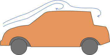
The automobile is different again, being short and squat. There is a significant discontinuity between the hood (bonnet) and windscreen, and in many cases a similar discontinuity at the rear window too (figure 15): both cause separation that in turn generates vortices. A further drag contribution arises from the wheels, which churn up the fluid flow inside the wheel arches, and another from the confused flow pattern under the floor pan. Less important are the wing mirrors, door handles, gaps round the doors and beading round the windows which are never quite flush with the outer body panels. For a modern family saloon, the value of the drag coefficient usually lies between 0.25 and 0.3 so we’ll assume a representative value of 0.28 at a cruising speed of 120 km/h. The value for a sports car is usually about the same, while that for a Formula 1 racing car is considerably greater. The reason is that high-performance cars are expected to produce downforce. Downforce improves the grip of the tyres on the road, but it’s created at a cost: induced drag (you might want to turn back to Section F1816 for an explanation of induced drag).
Figure 16
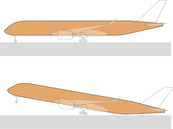
Finally, aircraft are aerodynamically more efficient than virtually all other vehicle types. The most bulky part of a passenger airliner is the fuselage, which is shaped like a zeppelin in elongated form with a rounded nose and a pointed stern, although the rear of the fuselage is canted upwards to allow the aircraft to take off without scraping its tail on the runway (figure 16). The cross-section of the wings also follows an elongated zeppelin profile, as does the cross-section of the rudder and tailplane. All have relatively smooth surfaces. Among the less ‘streamlined’ elements that contribute to drag are the engine nacelles, antennae, the undercarriage housing, gaps around the hinged control surfaces, and the housings for the hydraulic control surface actuators. Our archetypal model for passenger airliners must be the Boeing 747, the most successful of its kind ever built. The manufacturers of commercial aircraft don’t readily disclose details of their aerodynamic performance, but a few years ago, Professor David Mackay quoted a drag coefficient of around 0.031 in level flight at cruising altitude and speed [17]. It is based on frontal area. I have not been able to verify this figure, but I’ll use it anyway.
Figure 17
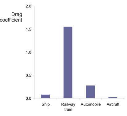
The drag coefficients for these four vehicles are plotted together for comparison in figure 17. The most striking feature is the high \(C_D\) value for the railway train, around fifty times greater than the value for the Boeing passenger jet. Does this mean that in comparison with other vehicle types, the railway train is fifty times less aerodynamically efficient?
Drag coefficients can be misleading
The problem is that we are trying to compare bodies of widely differing proportions, and the drag coefficient isn’t an appropriate way of doing it. Let’s look again at the classical drag formula derived in Section F1817:
(1)
\[\begin{equation} \text{Drag or resistance } D \quad = \quad \frac{1}{2} \rho V^{2} A C_D(\text{Re, Fr, Ma}) \end{equation}\]in which \(\rho\) is the fluid density, \(V\) is the vehicle speed, and \(A\) is the reference surface area. The braces on the right hand side indicate that depending on the circumstances, \(C_D\) may be a function of the parameters listed (the Reynolds number, the Froude number, and the Mach number), either singly or in combination. The parameters are usually taken as understood, so we’ll re-write the equation in the more familiar form:
(2)
\[\begin{equation} D \quad = \quad \frac{1}{2}\rho V^{2} A C_D \end{equation}\]To make comparisons across vehicle categories, we must interpret \(A\) in a consistent way, and in vehicle technology it is usually defined as the cross-sectional area viewed from the front. But this leads to a problem. Suppose we have two vehicles whose drag coefficients are both equal to 0.5. Given that they are travelling at the same speed, you might assume that their body shapes are equally efficient. But in the transport context, this doesn’t really help and can be misleading. ‘Efficiency’ is a way of comparing input and output. In the present context, the input is fuel and the output is the movement of passengers and goods: ideally, we want a measure of the fuel consumed per unit of travel, usually with travel measured in terms of passenger-kilometres or tonne-kilometres of cargo. As conventionally defined, the drag coefficient goes some way towards this, but falls short. What it actually measures is resistance per unit frontal area. The resistance is a good proxy for the input (fuel consumption), but the frontal area is not a good proxy for the output. Vehicles are not advertising hoardings and we don’t design them to maximise the amount of frontal area they carry along our roads.
A better basis for comparison
The value of \(C_D\) is useful for assessing the relative performance of two vehicles only if they have similar geometrical proportions. You might use it to compare two different models of a passenger saloon car, or two different versions of a 200-seat passenger aircraft, but not to compare a saloon car with an aircraft. What we are really care about is their performance as alternative ways of carrying an equivalent payload, for which a better yardstick would be the drag per unit volume. Suppose we want to re-design a particular vehicle to make it more aerodynamically efficient. Assuming that the payload is sufficiently flexible to fit into a long and narrow hold, we might be able to reduce the drag per kilogram of cargo or per passenger by reducing the frontal cross-section and stretching the vehicle lengthways, even if the drag coefficient - as conventionally defined - rises.
To establish a suitable yardstick, let’s re-arrange equation 2 thus:
(3)
\[\begin{equation} C_D \quad = \quad \frac{D}{\frac{1}{2} \rho V^{2}A } \end{equation}\]and define a new kind of ‘drag coefficient’ \(C_{new}\) such that
(4)
\[\begin{equation} C_{new} \quad = \quad \frac{D}{ \frac{1}{2} \rho V^{2} \nabla } \end{equation}\]where \(\nabla\) is the volume displacement. Effectively, \(C_{new}\) measures aerodynamic efficiency in terms of drag per unit volume. Unlike the original drag coefficient, it is not a dimensionless quantity, but we can easily make it so if we replace \(\nabla\) by \(\nabla^{2/3}\) thus:
(5)
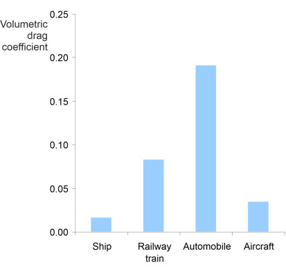
\[\begin{equation} C_\nabla \quad = \quad \frac{D}{\frac{1}{2} \rho V^{2} \nabla^{2/3}} \end{equation}\]For the sake of argument we’ll call \(C_\nabla\) the ‘volumetric drag coefficient’. It’s not a new concept, in fact it was introduced during the early part of the last century by engineers involved in airship design [14]. Values of \(C_\nabla\) for each of our four types of vehicle are listed in table 4 and plotted in figure 18.
| Vehicle category | Details | Volume displacement \(\nabla\) (m3) | Volumetric drag coeff \(C_\nabla\) |
|---|---|---|---|
| Ship | M4 Bulk cargo carrier | \(73910\) | \(0.017\) |
| Train | ETR 500 passenger train | \(2445\) | \(0.084\) |
| Automobile | Medium family saloon (Europe) | \(5.50\) | \(0.190\) |
| Aircraft | Boeing 747 passenger jetliner | \(2000\) | \(0.035\) |
The volumetric drag coefficient provides an alternative way to compare body shapes across the transport field. Seen through this lens, the value for the passenger train no longer appears as an extreme outlier, and interestingly, the ship emerges as a hydrodynamically more efficient body shape than the passenger jet, presumably because it has a simpler profile with no wings to generate frictional resistance or induced drag. The autmobile comes off worst.
Figure 18
Conclusion
With the exception of cargo ships, vehicles are moving faster today than they have ever done. But the faster the speed, the more fluid resistance they must overcome, so designers need to optimise the shape of the body shell. Of all the basic forms, the teardrop is the one with the lowest drag coefficient, but for land vehicles and sea-going vessels, other shapes are better suited to carrying passengers and cargo. We have seen how a degree of streamlining can help: rounded edges, smooth flanks, and a moderate degree of taper towards the rear can turn a rectangular box into a more aerodynamically efficient profile. When we compare vehicles across our four main categories, not surprisingly it turns out that our aircraft has the lowest drag coefficient. More surprising is the wide range of variation among the other three categories, with the drag coefficient for the railway train featured in table 3 around 50 times larger than the corresponding figure for a passenger airliner. This doesn’t mean that the railway train is fifty times less efficient, but rather, it reflects the way the values in the Table are calculated. If we re-define the reference area as \(\nabla^{2/3}\), the ratio falls from 50 to 2. Later in Section F1317 we’ll look at the question from another angle, and tackle a closely related issue, that of scaling. Given any particular shape for a body shell, how does its aerodynamic performance vary with size: are two small vehicles better than a single large one?
Figure 19

Acknowledgments
Photo on title page: An art piece Il futuro sta arrivando (the future has arrived) commissioned by an advertising agency in Milan in 2010 promoting the ability to create viral internet marketing through social media, and featuring in the journal Repubblica, source unknown.
Figure 03: ‘Intricate’ by Susanna Rosti Rossini.
Figure 07: Spats fitted to the Steen Skybolt G-BVXE, the 1998 Air Squadron Trophy winner, photography by Ed Hicks and Trevor Reeve as featured in Popular Flying, 11/12 1998, p32 in an article By Ed Hicks, available at http://www.steenaero.com/articles_detail.cfm?ArticleID=457 (accessed 05 May 2019).
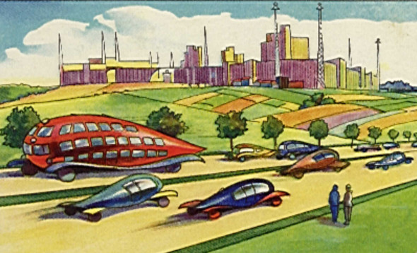
Figure 09: One of a series of trade cards distributed by Echte Wagner Margarine in the 1930s depicting ‘Vehicles of the future’.
Figure 19: Photo modelled by Cecily Hargreaves-Wright.