F.1816
Drag, lift & directional stability
The next time you ride on a bus, sit at the front and try to visualise what is happening outside. Not in the road ahead, but just beyond your window. The bus will push aside a lot of air before you reach your destination, and some of the particles are streaming across your line of vision a few millimetres away from the glass, maybe upwards, maybe to one side. We saw in Section F1817 that several kinds of force may be operating among the particles: they arise through different physical processes and ultimately are transmitted to the vehicle in the form of normal pressure and frictional forces that vary from place to place on the body surface. The aim of this Section is to see how in combination, these forces affect the vehicle’s motion.
Forces in three dimensions
We’ll deal with the forces under three main headings: drag, lift, and other forces. Drag is a cost: it slows the vehicle down, adds greatly to the fuel consumption, and probably limits how fast it can go. Lift is different. Although land vehicles don’t need it, lift is essential for aircraft to fly. Ships, too, need support from the surrounding fluid in the form of buoyancy, which for the moment we’ll regard as a kind of ‘lift’ although the mechanism is different. The third category includes several forces that we’ll come to in a moment.
Figure 1
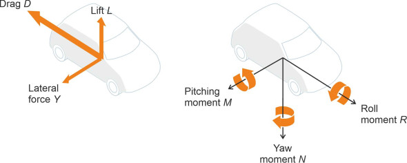
The six components
Next, we’ll map the forces onto a three-dimensional Cartesian framework as shown in figure 1. Further details are listed in table 1, where you’ll see that in total there are six distinct components, three forces and three couples. The notation differs among different branches of transport engineering but we shall follow the convention used in [22]. The first three lines of the Table refer to forces of the kind that push the body in a particular direction. We’ve already mentioned lift and drag; side forces arise whenever the fluid in which a vehicle is immersed arrives at an angle to its direction of motion. Whenever they turn, ships and aircraft use side forces to supply the centripetal acceleration they need to hold them on a curved path.
| Force or couple | Symbol |
|---|---|
| Lift | \(L\) |
| Drag | \(D\) |
| Side force (positive to starboard) | \(Y\) |
| Pitching moment | \(M\) |
| Rolling moment | \(R\) |
| Yawing moment | \(N\) |
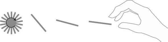
The last three lines in the Table are ‘couples’ or ‘moments’ that cause the vehicle to rotate. The pitching moment is particularly important in aircraft flight. On its own, an aircraft wing is unstable because the lift force is concentrated ahead of its centre of mass, near the leading edge. If you take the wing off a glider and catapult it into the air, the leading edge will pitch upwards and the wing will flip over onto its back and continue to rotate out of control. You can test this for yourself using a flat strip of cardboard or a plastic ruler as shown in figure 2.
Figure 2
Rolling moments are important for land vehicles and water vehicles. When a road vehicle or a railway train travels round a curve, it tends to roll around its longitudinal axis and topple over. This is caused by centrifugal force rather than fluid pressure, but fluid pressures are involved in the rolling motion of a ship under the impact of waves arriving on either the port or starboard side. Fluid forces also come into play when an aircraft banks or rolls, a deliberate manoeuvre by the pilot using the ailerons attached to the aircraft wings.
In the last line of the Table we have the yawing moment. When a vehicle yaws, it rotates about a vertical axis and therefore changes direction. Road vehicles steer by pivoting the front wheels, and railway trains are guided by the rails, but they sometimes experience aerodynamic yawing moments when travelling at speed in a cross-wind. Mostly they’re a nuisance, but at worst, they can upset steering and directional stability. On the other hand, ships and aircraft create yaw and lateral thrust artificially using rudders that deflect the fluid stream to one side: they are among the control forces that enable them to turn or hold a steady course.
Representing the forces and couples
Whenever it moves, a vehicle will experience a complex pattern of fluid pressures and shear stresses spread over its body surface that we can conveniently represent in shorthand form as the three forces and three couples listed earlier in table 1. But mathematically speaking, forces and couples are not independent. To explain why, we’ll picture a ship moving steadily through calm water, and consider only those agencies that affect its motion in the horizontal plane. The fluid pressures and shear stresses acting on the sides of the hull will push it bodily in a particular direction and at the same time, make it swing or rotate around a vertical axis. Call the thrust \(F\) and the couple \(M\). The question is how to represent these two actions on a piece of paper. In the leftmost diagram of figure 3, we depict the force \(F\) as a vector arrow; it defines the angle of \(F\) relative to the body’s longitudinal axis together with the line along which it acts. We represent the couple \(M\) with a curved arrow that shows whether it acts in a clockwise or anticlockwise direction. It doesn’t matter where the curved arrow is located on the diagram.
Figure 3
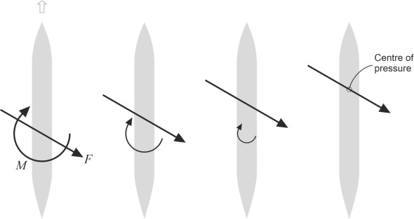
This representation is not unique. As shown in the next diagram to the right, we can shift the force to a new location closer to the bow, and adjust \(M\) so that their net effect remains unchanged. Suppose the new location of \(F\) lies a perpendicular distance \(h\) away from the original line of action, while preserving the value of \(F\) and the angle at which it meets the ship’s centreline as before. The force \(F\) now exerts a couple \(F\) around the original location, so we must reduce \(M\) to a new value \(M - Fh\) at the same time. If we carry on moving \(F\) forward in this fashion we can reduce the couple to zero, and dispense with it altogether. The final location of the line of action of \(F\) where it crosses the ship’s centreline is sometimes referred to as the centre of pressure, the place where the distributed pressures effectively act. In this way, we can represent the fluid load as a single vector quantity \(F\), but the results will sometimes look peculiar. Take, for example, the longitudinal cross-section of an aircraft wing: typically, the centre of pressure lies well forward of its mid-chord, and the resultant force may not actually pass through the wing at all [17].
Drag
Drag is almost always a nuisance. In the case of a family car at cruising speed, aerodynamic drag accounts typically for three-quarters of the total resistance [20]; the proportion is slightly greater for a high-speed train [13], and it’s 100\(\%\) for flying machines. Under most circumstances the drag increases as the square of the vehicle speed, so if you go twice as fast the engine will need to overcome four times the resistance.
Components of drag
Engineers like to break down the drag into constituents that arise from identifiable sources. The constituents don’t correspond to the force mechanisms described in the previous Section (F1817) but instead, they reflect (i) how the force is delivered to the body surface (i.e., normal pressure or shear stress), (ii) which part of the vehicle they act on, and (iii) its function. The labels used to identify different components – and indeed groups of components - differ among the various fields of vehicle engineering, and even among textbooks within the same field. Here we’ll attempt a compromise. A diagram of the main drag components appears in figure 4. Drag components that are delivered to the vehicle skin via shear stresses are highlighted in yellow, while those delivered via normal pressure are highlighted in red. Not shown in the diagram is wave-making resistance for ships. Nor are two of the components that affect aircraft, parasitic drag and interference drag; they are not distinct categories of drag, and we’ll deal with them separately later. So let’s examine the different components and try to understand their practical significance for different kinds of vehicle.
Figure 4
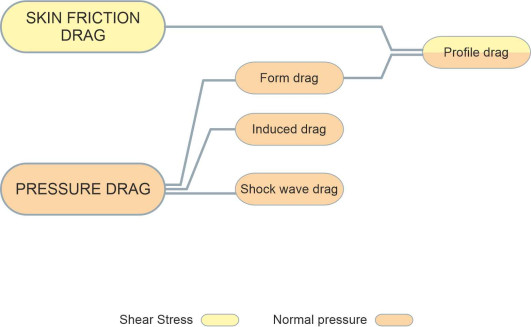
Friction drag
As its name implies, friction drag arises from the tangential shear stress exerted by a fluid in contact with the surface of a moving body. It is the chief component of drag for insects and birds, whose flight is characterised by relatively low Reynolds numbers. At intermediate Reynolds numbers, friction drag is less important, but still significant for railway trains and ships because they have a large surface area. On the other hand, the frontal area is small, so that any pressure difference between the front and rear doesn’t produce a large retarding force [9]. By comparison, an automobile is short and bluff so the contribution of skin friction drag is quite modest, less than a third of the total depending on the underbody design and body surface detailing [21]. For vehicles like jet aircraft that travel at high Reynolds numbers, the pressure drag dominates, and above the speed of sound, the greater proportion derives from shock waves.
Pressure drag
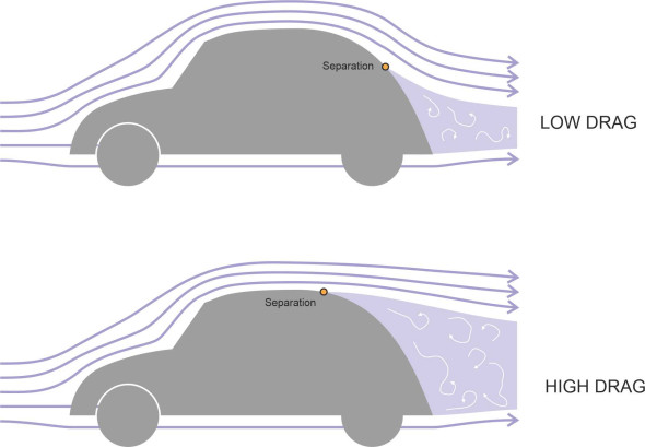
The term ‘pressure drag’ is interpreted differently in different fields of vehicle engineering. Here, we’ll use it as a generic term for any resistance component that is transmitted to the vehicle skin through normal pressure. This includes three sub-categories: form drag, induced drag and shock wave drag, all of which arise through different mechanisms but all of which are transmitted to the moving body in the same way. Form drag is usually the most important constituent, and it tends to dominate the others at moderately high subsonic speeds. (Confusingly, aeronautical engineers often use the term ‘form drag’ to denote all three components, i.e., as an alternative to the term ‘pressure drag’, while some marine engineers use a different term altogether [10].) It derives from the difference in normal pressure between the front and rear of a moving body, where the pressure is reduced because of the turbulent wake. This in turn is caused by separation of the boundary layer, so as shown in figure 5, the amount of form drag depends on where the separation takes place. It’s particularly important for road vehicles, so where possible the body is tapered to delay separation towards the rear where the cross-sectional area is small.
Figure 5
The concept ofinduced drag plays an important role in aircraft flight, but it can also be applied to boats that are supported by a dynamic interaction with the water surface such as planing craft or hydrofoil craft. Crudely, the idea is that a vehicle can obtain lift from the fluid through which it is moving by accelerating some of the fluid particles downwards. But there is a price. The kinetic energy imparted to the particles represents an energy drain that is reflected in a distinct component of drag. For aircraft, the induced drag has been called the ‘drag due to lift’, and it accounts for roughly a quarter of the total drag for a jet airliner [2]. It acts through pressure differences on the wing surface, and we’ll be looking at this more closely in later Sections. Here, we’ll focus not on the aircraft but on what happens in the surrounding fluid.
Figure 6
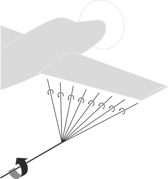
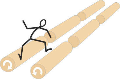
One might readily imagine that if the onrushing air is holding the machine up, the machine must be deflecting the air down, and while this is true, it’s not the whole picture – nor, for that matter, the most interesting part. The air passing under an aircraft wing tends to spill around the wingtip to the low-pressure region above, and in doing so, forms a vortex. It is part of a three-dimensional system, an extension of the circulation pattern around each wing that is drawn laterally outwards to the wing tip and left behind the aircraft in the form of a trailing vortex as shown diagrammatically in figure 6. If you think about it, air at subsonic speeds is more-or-less incompressible and if you push it down in one place it must rise elsewhere, so the net ‘downwash’ is zero. Hence the impact of the wing on the fluid particles is translated into angular momentum, not linear momentum. Imagine a lumberjack whose job is to manage some logs floating in a lake. They are arranged end-to-end in two parallel lines as shown in figure 7. The lumberjack starts at the near end, with his left foot on the first log on the left and his right foot on the neighbouring log on the right. Now, the weight of his left foot is slightly off-centre so the left-hand log begins to rotate clockwise as seen from the near end of the line. Similarly his right foot is bearing on the right-hand log, which starts to rotate anti-clockwise. The lumberjack doesn’t want to fall into the water between the logs so he walks forward. With each footstep the two logs roll faster, so he breaks into a run and leaps onto the next pair of logs and repeats the process, leaving behind a trail of rotating tree trunks. As long as there are more trunks to step onto, he can stay out of the water - it’s hard work but better than getting wet. In a similar way, an aircraft wing creates lift not by pushing the air down, but making it rotate.
Figure 7
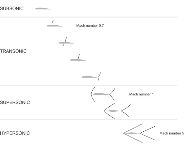
Shock wave drag is easier to understand. As described in the previous Section (F1817), when fluid particles pile up against an aircraft moving faster than the speed of sound, they create a zone of high pressure wrapped like a cloak around the leading edges of the wings and fuselage that greatly increases the resistance to motion. For a fluid particle entering this zone, the change in pressure is very abrupt: we call it a shock wave. Shock wave drag is one of the main sources of drag in supersonic flight, and it doesn’t scale in the same way as other forces because the geometry of a shock wave varies in a complicated way with the velocity of the aircraft. There are four distinct flow regimes [1]:
- Subsonic flow
- Transonic flow
- Supersonic flow
- Hypersonic flow.
In figure 8 you can see how the shock wave system develops as the Mach number rises [1] [19]. Picture the aircraft as stationary with the air moving past it. Initially, the air flow is subsonic throughout the flow field. However the fluid velocity varies around the skin of the vehicle: for example it will normally be higher over the top of an aircraft wing than underneath. As the pilot increases power and the aircraft accelerates, the air moving over the upper surface will reach the speed of sound and a local shock wave will form even though the aircraft itself hasn’t yet reached supersonic speed. This signals a change in behaviour of the wing, and the speed at which it occurs is call the critical Mach number Macrit.
Figure 8
At this critical point, the shock wave causes the boundary layer over the upper surface of the wing to separate. The separation leads to a fall in lift together with greater drag. For this reason, even though they can’t travel faster than the speed of sound, commercial jet airliners have to overcome significant wave drag when cruising at high altitude. Typically, the shock wave drag accounts for 20 – 30\(\%\) of the total [18].
Figure 9
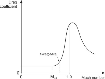
Military aircraft go faster. At velocities approaching Mach 1, the shock wave pattern changes and compressibility effects begin to dominate. The effect on drag is dramatic. At a speed slightly greater than Macrit called the ‘drag divergence number’, it rises sharply as shown in figure 9, and may increase by a factor of 10 [4]. Meanwhile, the lift falls, the aircraft tends to pitch nose-down, and rapid oscillations of the shock wave pattern cause buffeting. Once the aircraft is flying well above the the speed of sound, the drag coefficient falls again (but not to its original value) and the lift recovers. Learning how to break through this ‘sound barrier’ was one of the great challenges of 20th century aircraft design.
Other categories
Besides friction drag and pressure drag, there are other categories of resistance but they don’t involve new forces, only the ones mentioned earlier albeit grouped together in different ways. The first is profile drag: a term mostly used in connection with wind tunnel tests, in which aerofoil cross-sections are routinely evaluated using scale models that stretch from one side of the tunnel to the other so there are no trailing vortices. The resulting drag measurement represents skin friction and form drag but excludes induced drag. Another term used by aerodynamicists is parasitic drag. This is just the total drag with the induced drag component omitted. Its significance lies in the fact that induced drag in some sense is unavoidable, being essential for the aircraft to fly. The remainder, the ‘parasitic’ component, is not.
A third term used in the aeronautical field is interference drag. A streamlined vehicle can be pictured as collection of parts each of which affects the fluid flow. For example, an aircraft has wings, a fuselage, a tail unit, and engine nacelles, together with antennae and other ‘excrescences’ all of which contribute to lift and drag. To create a successful design, the engineer will break the problem down into its constituent parts and analyse the hydrodynamic contribution of each part separately as if it were moving through the fluid (air or water) on its own. In reality, however, the fluid flows around the various parts will interact with one another in such a way that the total drag works out larger than the sum of resistances estimated for each part separately. The difference is called ‘interference drag’.
Figure 10
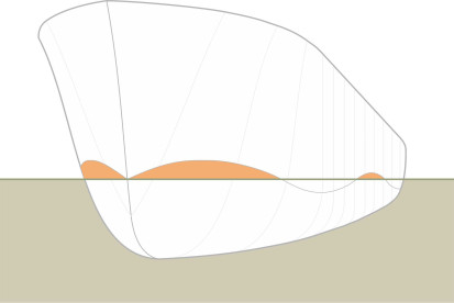
Finally, there’s a special category of drag that arises when a disturbance in one fluid medium spills over into another. A ship cleaves the water under the bow and forces the fluid particles apart. The pressure disturbance spreads outwards from the point of impact and when it reaches the surface, it creates waves that draw off energy. The energy loss signals a particular form of drag whose magnitude depends on the height and wavelength of the waves. If the ship were completely immersed like a submarine, say 50 m below the water surface, the disturbances would not reach the surface and the wave drag would be zero – in this respect a submarine is more efficient than a surface vessel! Although small at low Froude numbers [25] [26], the wave-making drag increases rapidly with the vessel’s speed, the relationship with speed being rather a complicated one (see Section M1620 and M1619). As shown in figure 10, the resistance component is probably delivered through differences in normal pressure acting on either end of the ship’s hull, because the water surface piles up against the bow and forms a trough at the stern. The impact depends partly on the geometric form of the bow: a blunt shape will have a more severe effect than a ‘fine’ one.
Lift
Fluids such as air or water resist movement, and by slowing down trucks and aircraft they add significantly to the rate at which the vehicles consume fuel. But fluids can also provide support. A cargo ship relies on the pressure of seawater spread over its hull to carry the vessel together with its payload of maybe 100 000 tonnes, and its buoyancy does away with the need for a supporting track. Water is not the only fluid that will provide support. Archimedes’ principle tells us that any gas or liquid will exert an upward thrust on a body equal to the weight of fluid it displaces, so that the air will carry a balloon, for example, high into the stratosphere. Buoyancy is the simplest of the gravitational force mechanisms, a ‘static’ force that operates whether or not the vehicle is moving and which is broadly independent of its speed. But most flying machines are heavier than air and rely on a different mechanism: they use motion to generate lift.
Dynamic lift
By comparison, aircraft have to work hard, using their forward speed to obtain lift from the air flowing over their wings, but at the same time they encounter less resistance than most other vehicles at any given speed. To work at all, the wings of an aircraft must deflect the air flow around them. The idea is to force it downwards, which generates an equal and opposite reaction, and it’s the reaction that keeps the aircraft flying. How much air must the wings deflect? Force equals mass times acceleration, and since a cubic metre of air doesn’t have much mass, in order to support the 400 tonne weight of a modern passenger jet the wings must accelerate large volumes of air and do it very quickly. How they manage this is not easy to explain in simple terms. There are several different explanations, and they work on different levels ranging from mathematical models to ‘mind pictures’ based on intuition and common sense. We’ll review some of them in Section A2020, but to pave the way, let’s examine the behaviour of the simplest possible form of wing, a flat plate aligned at a small angle to the oncoming air flow. Without actually doing any maths, the aim will be to show that a lift force must be present.
Assuming the flow is non-viscous, let’s start with the plate aligned perpendicular to the fluid stream as shown in the diagram at the top of figure 11. There are two stagnation points marked with an ‘S’, one at the centre of the upstream face and the other at the centre of the downstream face. At a stagnation point, Bernoulli’s law tells us that the dynamic pressure is zero so the static pressure must be at a maximum. The flow pattern is symmetrical about the \(x\)-axis, and where the flow curls around the upper and lower edges of the plate you will see the streamlines are bunched closely together, indicating regions where the pressure is at a minimum. Now rotate the plate anti-clockwise until the angle of incidence reaches a value of around \(20^{\circ}\) as shown in the diagram at the bottom; the upper edge moves forward and becomes a recognisable ‘leading edge’ while the lower edge moves aft to become a ‘trailing edge’. The rotation has three main consequences. First, the upstream stagnation point migrates towards the leading edge. Second, the downstream stagnation point migrates towards the trailing edge. Third, the streamlines are still bunched together over the upper surface at the front and the lower surface at the rear, so the two low-pressure zones persist, one above the leading edge and one below the trailing edge. With the plate aligned at the angle shown, the first produces an upward force on the plate and the second a downward force.
Figure 11
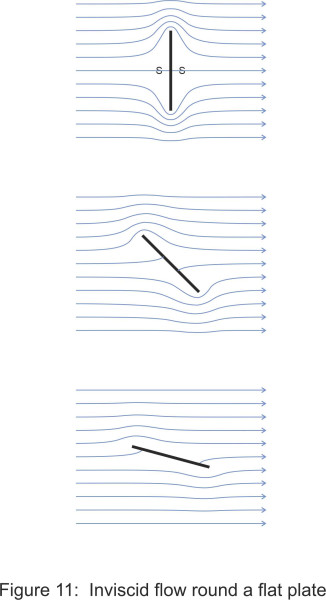
However, the plate isn’t producing any lift yet - the forces balance out. Imagine two fluid particles, the first one, labelled ‘U’, passes along the upper surface of the plate. The second we’ll label ‘L’; it passes along the lower surface. Both journeys start at the forward stagnation point and terminate at the aft stagnation point, and in between both particles follow an inclined path and curl around a sharp edge. Considerations of symmetry suggest that the upward force and the downward force are equal and opposite in direction and while they generate a net couple that we’ll examine later, the net vertical force is zero. But we’ve overlooked an important detail. The pattern is not symmetrical but anti-symmetrical, which means that the two particles experience the same events but in a different order. For a non-viscous fluid this doesn’t affect the outcome, but for a viscous fluid it does.
To see why, it helps to picture each particle as having an energy budget. For the moment we’ll ignore any friction effects. Both particles start off from the forward stagnation point at the same time, each having zero velocity and zero kinetic energy. First we’ll trace the journey of particle U. It starts from a region of high pressure, and the pressure gradient propels it towards the low-pressure area around the leading edge. During the process it acquires kinetic energy. After curling round the leading edge, the particle begins to slow down again because it is working against an adverse pressure gradient and it is losing kinetic energy along the way. When it arrives at the aft stagnation point, its kinetic energy has dissipated completely and it comes to a halt. Figuratively speaking, there’s ‘nothing left in the tank’. Meanwhile, particle L has completed a similar journey underneath the plate, and arrives at the aft stagnation point and comes to a halt at the same moment.
So now we’ll make the fluid ‘real’ by giving it non-zero viscosity, and see what difference this makes to the flow pattern. Moving in contact with the upper and lower faces, the particles U and L together with all the nearby particles in their respective boundary layers will undergo frictional shear stress and will lose kinetic energy more quickly than would otherwise be the case. What will happen to them? We know that if a boundary layer stops, it will separate from the surface of the plate. The result is shown in figure 12. The ‘upper’ flow encounters the sharp leading edge while it still has plenty of energy. It curls round the edge at speed, breaking away momentarily before re-attaching itself downstream. Only afterwards does the kinetic energy dissipate as the boundary layer undergoes friction along the upper surface of the plate. By contrast, the ‘lower’ flow undergoes friction and loses momentum before it reaches the trailing edge, and herein lies the key. It can no longer reach the aft stagnation point because it has lost the kinetic energy it needs to curl round the trailing edge against an unfavourable pressure gradient. At this point it breaks away.
Figure 12
Finally, we can return to particle U. The aft stagnation point has effectively vanished and no longer blocks the way, so the upper boundary layer can keep moving and join smoothly with the lower one aft of the plate as shown in figure 12. A smooth reconciliation at the trailing edge is the essence of the Kutta condition that lies at the heart of airfoil theory. It’s an assumption that seems to be borne out in practice. With the blockage removed, the upper boundary layer moves faster than the lower one and the pressure on the upper surface is reduced – there is a net upward lift. You can see this reflected in the fluid streamlines, which angle downwards slightly as they pass across the flow field from left to right, implying that the plate is pushing fluid downwards. With a little imagination, you can also visualise a degree of ‘circulation’ around the plate which arises from the higher particle velocity over the upper surface. As theoretical analysis will confirm later in Section A1716, downwash and circulation are defining characteristic of airfoil behaviour. In a curious way, it’s the friction that brings about asymmetry and causes lift.
Figure 13
Real wings are aerodynamically more sophisticated: their cross-sectional shape has evolved with a curved outline to achieve (among other things) a smoother flow pattern with more lift and less resistance (figure 13). The outline is not symmetrical, and in particular, the upper surface is more rounded than the lower surface, a feature known as camber. The streamlines passing over the top are squeezed together more tightly than those passing underneath, which implies a higher speed and therefore (according to Bernoulli’s theorem) lower pressure. The particles also experience centrifugal force, which further lowers the pressure and encourages a higher velocity. The two effects – reduced pressure and increased velocity - reinforce one another with the result that, compared with the flat plate, a properly designed airfoil section produces considerably more lift with less drag.
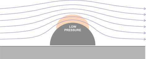
Cars can fly too
A road vehicle produces lift, although this may not be the designer’s intention. Recall the example mentioned earlier in Section F1917 in which a circular cylinder was immersed in an inviscid fluid stream with its axis at right-angles to the oncoming flow. The flow pattern around the upper half of the cylinder is a mirror image of the flow pattern round the lower half. If we cut the cylinder horizontally in two as shown in figure 14 we can imagine the upper half as a ‘vehicle’ by placing it close to the ground so there is minimal flow underneath. The cross-section is semi-circular and the flow pattern over the ‘roof’ will be identical with the flow pattern over the upper half of the cylinder. We know that the velocity peaks around the summit and that in conformity with Bernoulli’s Law the pressure falls, so that assuming the pressure underneath equals the static pressure \(p_0\), there will be a net upward force. In fact, almost any road vehicle will generate a lift force in this way, and the faster it goes, the greater the lift. Over the years there have been several cases in which vehicles attempting to break the land speed record have actually left the ground, with fatal results. In the 1970s, the lift generated by a typical family car was almost as great as the drag, but racing car designers learned how to reverse the lift and create ‘downforce’ by manipulating the flow under the vehicle body, and adding aerodynamic ‘wings’ over the rear axle [6]. The aim was to improve the grip of the tyres so corners could be taken at higher speeds. At its peak, aerodynamic design produced Formula 1 cars whose downforce was roughly equivalent to four times the vehicle’s weight [12].
Figure 14
Added mass
Until now, we have imagined the pattern of flow round a moving vehicle as remaining steady over time, so that the forces on the vehicle body are constant. But what if the body is weaving from side to side, or bobbing up and down like a ship in a storm? Motions like this introduce a phenomenon that we haven’t yet considered. When the bow of a ship plunges into a trough, it rams the water and accelerates an appreciable mass of fluid downwards. The inertia of the water resists penetration by the hull, a phenomenon for which engineers have coined the term added mass. The fluid particles effectively damp the up-and-down motion, as signified by the additional waves that radiate outwards from the hull across the water surface [8]. The question is how to model the interaction: in simple cases one can estimate the mass of water involved and incorporate an extra term for the added mass in the equation of motion, but things gets more complicated for a ship whose hull doesn’t conform to a simple geometrical shape; you’ll find more about this in Section M1115, and a great deal more in the specialist literature [23].
Yaw
Drag and lift are examples of forces whose effect is to push a body in a particular direction. Provided it is not going too fast, neither the drag force nor the lift force greatly affects the way a vehicle handles. But other forces might. A crosswind can push a car sideways with a force whose magnitude depends on the body’s shape and may be greater than the drag [15]. Having rails to guide them, trains are less vulnerable to aerodynamic forces of this kind, although in theory an extreme gust might overturn a moving train [5], and in fact a train was once blown off the exposed Owercarrow Viaduct in Ireland. At sea or in the air, the effect of a transverse current is not usually dangerous except at the start or finish of the journey because the pilot can steer at an angle to its intended course and there is plenty of room for the vehicle to crab from side to side. As we’ll see later, what matters more is whether the fluid forces can make a vehicle change direction. In particular, a fluid can apply a couple or moment that causes it to rotate around any of the three axes shown earlier in figure 1. Rotation about the \(x\)-axis is called roll, while rotation about the \(y\)-axis is called pitch. Rolling and pitching motions can make travel uncomfortable as you’ll know from riding in a car with soft suspension, or sailing in a rough sea. But for now we’ll concentrate on yaw, which is rotation about the \(z\)-axis so that the vehicle changes direction. Compared with that of a lateral ‘push’, a couple that causes a vehicle to yaw is potentially more serious because when a vehicle changes direction it quickly departs from the driver’s intended path. How might this occur?
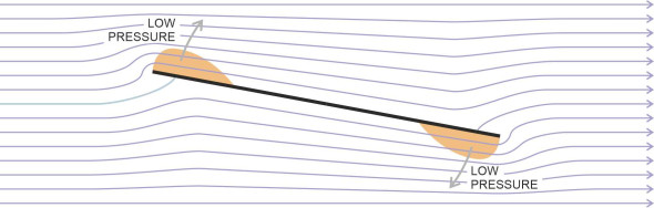
The Munk moment
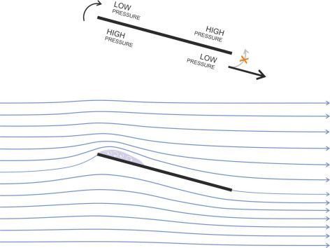
To answer this question it will help us to look again at the flat plate mentioned earlier. Recall that the plate is moving through an inviscid fluid. When aligned at an angle to the incoming fluid flow as shown earlier in the lower part of figure 11, it develops low pressure areas that occur where the fluid accelerates around the edges of the plate. The flow pattern is reproduced in figure 15, this time with the low pressure areas highlighted. They are located (i) on the downstream side of the leading edge and (ii) on the upstream side of the trailing edge [24], and together they exert a torque around the mid-point of the plate. The torque is called the Munk moment, after Max Michael Munk (October 22, 1890 – 1986), a German aeronautical scientist who studied under Ludwig Prandtl and worked briefly for the German Navy before emigrating to the USA during the 1920s. He drew attention to the phenomenon in his work on the stability of airships.
Figure 15
The Munk moment is a distinct phenomenon that occurs whether or not there are any lift or transverse forces acting on the body: it is a pure couple, and interestingly, it is self-reinforcing. If we change the orientation of the plate shown in figure 15 so it is aligned horizontally - exactly parallel to the oncoming flow – there will be no upward or downward forces and the couple will be zero. But the slightest angular deviation arising from a random disturbance in the air flow will lead to a Munk moment and trigger unstable behaviour. If the nose pitches up, the moment acts clockwise and with each increment of pitch, its magnitude increases. As shown in figure 16, the plate will rotate through an angle of \(90^{\circ}\) until it lies perpendicular to the direction of motion, when the symmetry of the flow field is restored and the moment returns to zero. This is a stable position and in principle, the plate will return to it if disturbed. However, you’ll recall that earlier, we claimed that a flat ‘wing’ made from a piece of cardboard would continue to rotate as shown in figure 2. This can happen if the plate’s angular momentum carries it beyond the stable position; once the angle passes \(180^{\circ}\) the process will start again and the rotation may continue through many cycles.
Figure 16

You might wonder how all this relates to the question of directional control. In figure 16 we are looking at the plate from side. But it can just as well represent a ship viewed from above, in which case the angular deviations can be interpreted as yaw angles. It seems that when floating in a liquid of zero viscosity, a long, thin ship cannot be directionally stable: it will tend to drift off-course. The same applies to a long, thin rod immersed in the fluid like a submarine, or flying through the air like an arrow. Frustratingly, it doesn’t follow the line of least resistance - unless it is equipped with stabilising fins, it will turn sideways on to the fluid flow.
Directional stability
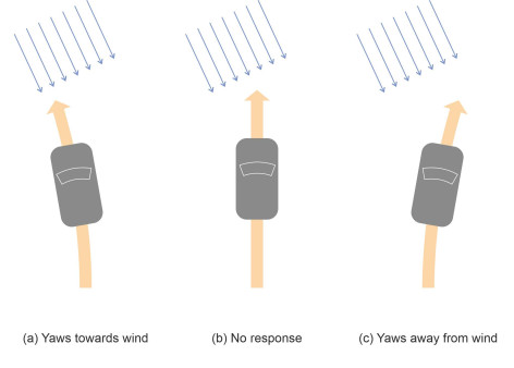
For a vehicle moving through a real fluid, the interaction between the fluid and the body surface is more complicated. There are forces as well as couples, so that when a vehicle encounters a lateral gust of wind, it will tend to move sideways as well as rotate. The designer wants the vehicle to handle safely in bad weather, and aerodynamic stability is an important consideration. But what does ‘aerodynamic stability’ mean? In a crosswind, as shown in figure 17 any one of three things can happen:
- The vehicle turns towards the oncoming flow like a weathercock, which lessens the severity of the disturbing forces,
- the vehicle continues to move in the same direction as if nothing had happened, or
- the vehicle turns away from the oncoming flow, which makes the disturbing forces worse.
Figure 17
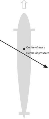
Which of the three outcomes will actually occur depends on the type of vehicle. If the vehicle is moving freely through a fluid without any track to guide it or any contact with the ground, the key factors are the ‘centre of pressure’ where the line of action of the lateral thrust crosses the longitudinal axis of the vehicle, and its relationship to the centre of mass. Suppose we are dealing with a submarine that runs into a current that crosses its path. If as shown in figure 18 the centre of pressure lies aft of the centre of mass the submarine will behave in a stable fashion as specified in (a) above – it will turn towards the source of the current and the destabilising force will diminish. Conversely, if the centre of pressure lies forward of the centre of mass, not only will the current push the submarine sideways, but it will rotate the hull away from the source so that the destabilising force grows in magnitude and the rate of yaw increases. This constitutes unstable behaviour as per outcome (c). For directional stability the centre of lateral pressure must lie aft of the centre of mass, which is most easily achieved by means of stabilising fins like those on a rocket ship, or simply a long tail like a javelin. The same applies to aircraft.
Figure 18
What about automobiles? Here the situation is complicated by the interaction between the wheels and the road. When a crosswind causes the vehicle to change direction, what happens next depends on three factors: (i) the location of the centre of lateral pressure (ii) the location of the centre of mass, and (iii) the suspension and steering. For most road vehicles the centre of lateral pressure is located well forward, about a third of the car’s length from the front [7] and a short distance behind the centre of mass [16]. In practice, with the centre of pressure located well forward, most road vehicles tend to turn away from the wind. In technical terms, this is aerodynamically unstable behaviour, but it’s easier for the driver to handle than outcome (a). The reason is that as well as making it yaw, a crosswind will usually push the vehicle to one side. Suppose the wind is coming from the car’s nearside. The vehicle will crab sideways towards the middle of the road. At the same time it will turn into the wind on a new course heading for the edge of the road. What should the driver do? One’s first reaction might be to steer away from the middle, which makes the yaw displacement worse and force the vehicle off the highway. In practice, most cars seem biased towards outcome (c), which enables the driver to handle the two sorts of deviation (lateral displacement and angular displacement) with a single and more intuitive response – by steering into the wind.
However the situation will change if the grip of the front tyres is appreciably better than the grip at the rear. The ‘slip angle’ of the rear tyres will be larger and they will crab sideways in a way that tends to exaggerate any steering corrections made by the driver. In this condition, the car is said to oversteer and as explained in Section C0418, it can become difficult if not dangerous to drive in a crosswind. You can find more about the interaction between steering and wind forces for a typical family car in [11] and [14].
The problem for ships is different. They interact with not one but two kinds of fluid: water and air, either of which can induce a form of directional instability similar to that associated with the Munk moment. First, let’s see what the water can do, assuming calm conditions with negligible wave action. If you think of the hull as a long, thin stick, when it yaws slightly, you would expect low-pressure areas to develop at the bow and stern that if unchecked, will rotate the hull so as to reinforce the rate of yaw. Most ships are designed so that the rudder and the ‘skeg’ (the fairing ahead of the rudder) constitute a sufficiently large area to ensure that the centre of pressure lies aft of the centre of mass. This will enable the ship to hold a steady course, but as described in Section M0418, cases have occurred where the ship is directionally unstable; to maintain a given heading, the helmsman must make continual adjustments otherwise the vessel will slew off to one side. The wind can also affect a ship’s heading, but with different results. If the engines fail in a storm, the aerodynamic forces on the superstructure can rotate the vessel until it lies broadside-on to the wind. It is now exposed to waves that can make the vessel roll heavily and even capsize.
Conclusion
In this Section, we have investigated the fluid forces that affect a moving vehicle. Fluid resistance is responsible for a major share of a vehicle’s fuel consumption, and limits the speed at which the vehicle can operate, while lateral forces together with yawing moments combine to influence handling behaviour. We are now quite close to deciding from an aerodynamic point of view what might be the ideal shape for a moving vehicle, if indeed such a thing exists. In Section F1616 we’ll examine some simple geometric shapes and compare their behaviour in an attempt to explain why vehicles take on the distinctive forms that they do.