© Harper's Young People
M.1115
Seakeeping
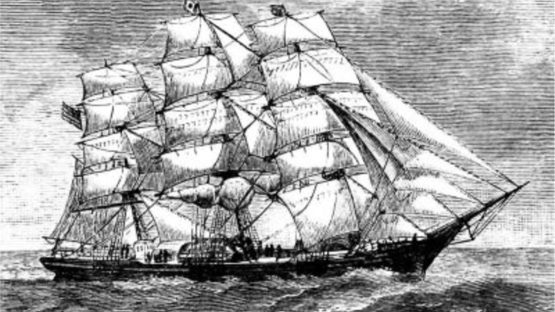
There is no shelter in the middle of the ocean. From time to time, a storm will raise waves that are taller than a ship’s mast. Vessels heave, pitch and roll for hours on end as waves batter the hull, sometimes breaking over the deck and threatening to damage the superstructure or even turn the vessel over. Building ships to withstand impacts of this kind poses a challenge to designers, one that distinguishes marine architecture from all other branches of transport engineering. In the past, shipwrights relied on experience and craftsmanship to produce vessels capable of surviving in all weathers. A notable example was the nineteenth century ‘clipper’ sailing ship. Clippers could navigate, for example, between the east and west coast of the American continent via Cape Horn, and race across the Indian Ocean to bring luxury goods from China to Europe. With their slender hulls, tall masts and square sails, the fastest could reach 20 knots and they broke records with every season. But it wasn’t just a question of speed: clippers could keep up a steady pace in conditions that would defeat other craft [5].
We use the term sea-keeping to describe how a ship responds to rough seas. It’s a trade-off between safety, strength and speed, and although there’s no perfect solution, designers have learned where the risks lie, what hull shapes work well, and which are the ones to avoid. But there is always pressure to develop new configurations, or stretch existing ones beyond familiar boundaries. It’s not easy to predict how a new design will respond to rough seas. You can get some indication of what is involved from [3] [12] or [17]. Here, we’ll try to explain the problem in everyday language, and indicate how designers are trying to solve it.
Motions at sea
One can think of the sea as a bumpy platform. The ship travels along the surface, rising and falling with the waves like a truck responding to bumps in the road. But unlike a road surface, the sea itself is continually in motion, changing its shape underneath the hull. To understand the ship’s behaviour, we’ll start by dealing with the motions separately, looking briefly at the sea first, then the different ways the hull can respond, before moving on to the relationship between the two.
Different kinds of motion
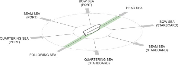
At sea, the waves can bear down on a ship from any direction, at an angle between \(0^\circ\) and \(360^\circ\) relative to the ship’s longitudinal axis. But for practical purposes, mariners divide the directions into eight main sectors; they are listed in table 1 and shown diagrammatically in figure 1.
| Name | Where the waves are coming from |
|---|---|
| Head sea | Directly ahead |
| Bow sea | Port quarter |
| Starboard quarter | |
| Beam sea | Port side |
| Starboard side | |
| Quartering sea | Aft port quarter |
| Aft starboard quarter | |
| Following sea | Directly astern |
Waves that arrive from different sectors have different effects. A beam sea will make a ship roll from side to side, while a head sea or a following sea will make it pitch. And in what follows, we’ll discover that the time interval between successive waves is important, because if it coincides with the natural period of oscillation of the hull, the ship’s motions can quickly get out of hand. But the time period as experienced by the hull is modified by the direction of the waves and the speed of the vessel. For example, in a head sea, the ship encounters more waves per unit time than would otherwise be the case so the period between successive crests is reduced. If we denote the phase velocity of the waves by \(V_w\) and their wavelength by \(\lambda\), and denote the velocity of the ship by \(V\), then from the ship’s point of view the waves are arriving at a relative velocity \(V_{w} + V\). However the wavelength is unchanged, so the period must be reduced by a factor \(V_{w}/(V_{w} + V)\). By contrast, in a following sea when the waves arrive from astern, the period increases by a factor \(V_{w}/(V_{w} - V)\). The longer period associated with a following sea turns out to be important, as we’ll see later.
Figure 1
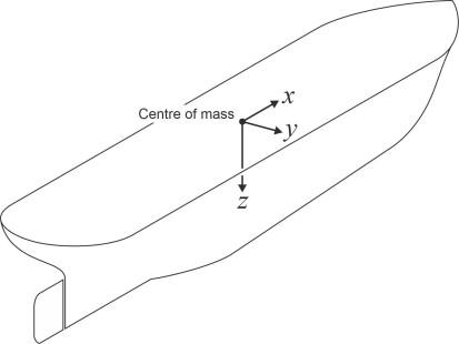
So how to describe the movements of the ship itself? The frame of reference is defined by three perpendicular axes as shown in figure 2 [11] [19]. It is similar to the one used for analysing the behaviour of land vehicles such as automobiles. The origin lies at the centre of mass, and the three axes are:
- \(x\) axis: aligned horizontally fore and aft along the ship’s centreline, positive in the forward direction
- \(y\) axis: aligned horizontally from side-to-side, positive to starboard
- \(z\) axis: aligned vertically, positive downwards.
Figure 2
Notice that it’s different from the system used by naval architects. Naval architects are concerned with building the hull, and they measure progress from the bottom upwards. They also relate their longitudinal dimensions to the stern post, so the origin of their coordinate system lies underneath the keel at the stern. Moreover, the sea-keeping frame of reference is not (strictly speaking) ‘attached’ to the ship, because it marks the ship’s position independently of whether the hull is disturbed by wave action: it is called the ‘reference parallel’ frame [7].
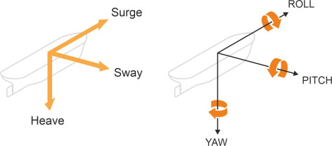
Within this frame of reference, the ship can move backwards and forwards in oscillatory fashion along its axis of symmetry; it will undergo small displacements from side to side and up and down as well, depending on the motion of the water surface. Such movements are called translations. It can also revolve about the axes singly or in combination: these are rotational movements, for example, spinning around its vertical axis like an ice-skater. Hence the motions of a ship, like those of a car, a railway vehicle, or an aircraft, can be broken down into 3 translations and three rotations, a total of 6 components. The translation movements are called surge, sway and heave, while the rotations are called roll, pitch and yaw. Note that at any moment, two or more may be acting simultaneously. The motions together with their axes are set out in table 2 and illustrated in figure 3. They are identical to the ones we used earlier in Section C1416 and Section G0216 in connection with the dynamics of road vehicles. The ones that passengers and crew notice are the ones that involve an oscillatory motion with a regular period: they are heave, pitch, and roll.
| Axis | Translation | Direction | Rotation | Direction |
|---|---|---|---|---|
| Longitudinal | Surge | \(x\) positive forwards | Roll | Around the \(x\)-axis, positive starboard down |
| Lateral | Sway | \(y\), positive to starboard | Pitch | Around the \(y\)-axis, positive bow up |
| Vertical | Heave | \(z\), positive downwards | Yaw | Around the z-axis, positive bow to starboard |
Figure 3
What follows is not a systematic exposition, but a few highlights to illustrate a complex field. Let’s start with heave, because it is the motion that easiest to analyse. When a small boat puts out to sea it will bob up and down with the waves in the same way that a baby’s push-chair traces out the bumps over rough ground. Like the baby, the dinghy sailor gets an uncomfortable ride. But a large ship is different. The water isn’t solid, and we expect the vessel to iron out some of the bumps as if cushioned by soft springs. Is this a realistic picture?
Figure 4
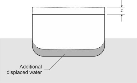
Heave
Imagine the ship is lying stationary in calm water. Let’s carry out a thought experiment similar to the one described in Section G1115 on a car suspension. We’ll force the vessel downwards into the water by a small amount (never mind how) and see how it responds. When the hull is released, it will rise again, but what happens after that? To keep things simple, assume that the sides are vertical near the waterplane. For any given deflection \(z\), the hull will displace an additional amount of water equal in volume to \(Az\) where \(A\) is the waterplane area (figure 4). This will momentarily increase the buoyancy, producing an out-of-balance or restoring upthrust \(F\) equal to \(-\rho g A z\) force units where \(\rho\) is the mass density of seawater (and \(F\) is negative because it’s in the opposite direction to \(z\)). Ignoring both the mass of the displaced water and the friction it exerts on the hull plating (we’ll return to them later) we can now invoke Newton’s Second Law (force equals mass times acceleration) and write down the equation of motion:
(1)
\[\begin{equation} - \rho A g z \quad = \quad M \times \frac{d^2 z}{d t^2} \end{equation}\]where \(M\) is the mass displacement. The restoring force on the left hand side is proportional to the deflection, which implies simple harmonic motion so the ship continues to oscillate like an automobile on its springs. After rearranging, equation 1 appears in the standard form
(2)
\[\begin{equation} \frac{d^2 z}{dt^2} + \frac{\rho g A}{M}z \quad = \quad 0 \end{equation}\]which can be solved to show that \(z\) follows a sine curve with fixed period \(T_H\) given by
(3)
\[\begin{equation} T_{H} \quad = \quad 2 \pi \sqrt{ \frac{M}{\rho g A}} \quad = \quad 2 \pi \sqrt { \frac{\nabla}{gA} } \end{equation}\]where \(\nabla\) is the volume displacement. The details are set out in Appendix 1. Equation 3 is important because if the sea turns rough and \(T_H\) happens to coincide with the time interval between wave crests, there will be resonance – in theory the hull will heave up and down over a range that theoretically increases without limit. You might find it interesting to compare it with the equivalent formula for an automobile suspension. As shown in Section G1115, if you mentally divide a car into four quarters and picture one of the quarters as moving up and down independently of the others, it has a natural frequency \(N\) in cycles per unit time whose value is given by
(4)
\[\begin{equation} N \quad = \quad \left( \frac{1}{2 \pi} \right) \sqrt{ \frac{kg}{P}} \end{equation}\]where \(P\) is the weight carried by that wheel measured in force units, and \(k\) the stiffness of the spring. By definition, the natural period of oscillation is just the inverse:
(5)
\[\begin{equation} T \quad = \quad 2 \pi \sqrt{ \frac{P}{kg} } \end{equation}\]A low value of \(k\) means a floppy spring, and a long natural period. It’s a ‘soft’ suspension. Now, the heaving motion of a ship can be construed in a similar fashion. Although the notation is different, for each variable in equation 3 there is a corresponding variable in equation 5: the ship’s mass displacement \(M\) corresponds to the wheel load \(P\), while the seawater density \(\rho\) times waterline area \(A\) corresponds to the spring stiffness \(k\). A deep, narrow hull (small area \(A\)) has a longer natural period than a shallow, flat-bottomed one of the same displacement (large \(A\)). This is presumably one of the reasons why the wave-piercing catamaran has become popular as a coastal ferry - it bobs up and down more gently in choppy waters (figure 5). This illustrates an important principle in sea-keeping. Generally speaking, the designer tries to make the natural period for a ship’s motion – any motion, not just heave – longer than the period of waves likely to be encountered in normal service, so that resonance doesn’t often arise.
Figure 5
We can glean something else from equation 3. Suppose we don’t want to change the shape of the hull, merely scale it up or down in size. Then the volume displacement \(\nabla\) within the square root sign on the right-hand side will scale in proportion to the length cubed \(l^3\), while the waterplane area \(A\) will scale in proportion to \(l^2\). Hence the period scales up or down in proportion to \(\sqrt{l}\): other things being equal, the bigger the ship, the longer the period. Let’s visualise a cargo ship Cecily of 35 900 tonnes displacement whose length is 175 m and waterplane area 3 500 m2. If we take the density of seawater as 1025 kg/m3, from equation 3 the heave period works out at 6.3 s approximately. If we now double the overall size of the hull while keeping all dimensions in the same proportion, the mass displacement increases to \(2^{3} \times\) 35 900 = 287 000 tonnes while the waterplane area increases to \(2^{2} \times\) 3500 = 14 000 m2. The period then increases to about 9.0 s. In other words, a big ship rises and falls more slowly. However, as we’ll see later, the heave period is influenced by two other factors that we have yet to take into account: damping through friction and the ‘added mass’ effect.
Pitch
When a ship heaves, the whole body is carried in a particular direction - up or down. Technically it’s a ‘translation’ from one position in space to another, and the motion involves familiar quantities like deflection, velocity, acceleration, and mass. But when it pitches or rolls, the motions are ‘rotational’. In purely rotational motion the centre of mass doesn’t move, and the the quantities of interest are now angular deflection, angular velocity, angular acceleration, and moment of inertia. In addition, the hull geometry is more complicated, and it’s more difficult to work out an expression for the natural period. Expressions for the natural period of both pitch and roll are derived in Appendix 2. The natural period \(T_P\) for pitching motions in still water is given by:
(6)
\[\begin{equation} T_{P} \quad = \quad 2 \pi \sqrt{ \frac{I_{yy}}{\rho g \nabla . \overline{ \text{MG}_{P}}}} \end{equation}\]where \(\nabla\) is the volume displacement, \(\rho\) the density of water, \(\overline{ \text{MG}_P }\) is the metacentric height relevant to pitching motions, and \(I_{yy}\) is the moment of inertia about the \(y\) axis. The latter is often written in the form
(7)
\[\begin{equation} I_{yy} \quad = \quad M . {r_{yy}}^2 \end{equation}\]The radius of gyration \(r_{yy}\) for pitch is commonly taken as one quarter of the ship length [6], which for a cargo ship of length 175 m works out at 43.75 m. Suppose that \(\overline{ \text{MG}_P}\) is around 50 m, then the natural period of pitch comes to about 12.4 s. In general, for ships of the same shape, the natural period scales with the square root of the hull length, so (as you might expect) a large ship pitches at a lower natural frequency than a small one.
Roll
Like the pitch period, the natural period of roll usually works out longer than the heave period, typically in the range 10 – 15 seconds for a displacement monohull in calm water. Imagine the ship is nudged momentarily by some external agency so it heels to one side through a small angle \(\phi\). When released, it rebounds, rotating in the opposite direction, passing through its original position, and continuing to oscillate as if under the influence of a torsion spring. In Appendix 2, we show that if added mass and friction are ignored, the natural roll period \(T_R\) for small deflections is given by
(8)
\[\begin{equation} T_{R} \quad = \quad 2 \pi \sqrt{ \frac{I_{xx}}{\rho g \nabla . \overline{ \text{MG}}}} \end{equation}\]where \(\overline{ \text{MG} }\) is the metacentric height in roll (here, we measure it positive downwards in the same direction as \(z\), although in most text books it is measured positive upwards and the result labelled \(\overline{ \text{GM} }\)). The quantity \(I_{xx}\) is the moment of inertia of the ship around its longitudinal axis, usually written in the form
(9)
\[\begin{equation} I_{xx} \quad = \quad M . r_{xx}^{2} \quad = \quad \rho \nabla . r_{xx}^{2} \end{equation}\]where \(M\) is the ship’s mass and \(r_{xx}\) is the radius of gyration, usually evaluated in metres. It is a time-consuming business to work out a reliable estimate of its value, and if you want quick results you can avoid the problem and instead use an empirical formula for the roll period, examples of which you can find in [20] and [14]. To get an idea of the numbers involved, your author applied both of these to estimate the natural roll period for the cargo ship Cecily mentioned earlier. Without going into detail, they gave approximately the same result, about 16 s.
Assuming that it’s a realistic estimate, we can now ask the key question: does it lie within the range of wave periods that the ship is likely to encounter, because if so, there is a risk of resonance together with large angles of roll. Crucially, the period between successive wave crests is usually less than 10s, so the risk is small. But in a quartering sea where the waves are arriving at a small angle on either side of the stern, the encounter period increases. It follows that with certain provisos, in a heavy sea the safest direction of travel is directly into the waves.
Forced oscillations
We now have three equations (equation 3, equation 6 and equation 8) that tell us how a ship might behave when jolted away from its equilibrium position in still water. The next step is to find out what happens when it is exposed to a regular train of waves; in particular, how it responds if the waves are in step with its natural period of motion. We are now dealing with forced oscillations: the waves inject a periodic disturbance as the height and slope of the water surface vary in sinusoidal fashion. In principle, the waves could be arriving from any direction, and they can excite many possible motions or combinations of motions. However, we’ll confine our attention to two cases. We’ll start with heaving motions in a head sea and then move on to rolling motions in a beam sea. In both cases we think of the wave motions as ‘input’, and observe the effect they have on the ship’s motions as the ‘output’.
Added mass and damping
In effect, we imagine the ship riding over the water in much the same way as an automobile rides over a bumpy road. A car has springs, which partially absorb the bumps and pass them on to the vehicle body as a smoothed-out ‘signal’ of reduced amplitude. The water underneath a ship cushions the hull in a similar way, but there are two differences. The first has to do with added mass. The water changes shape, but it can’t be compressed, so any motion that involves acceleration (as it would if the ship were heaving up and down) forces the water to accelerate too. Water has inertia and an additional force is needed to move it, so in effect, the ship has acquired extra bulk or ‘added mass’. It follows that when the ship moves in response to a given force, it will accelerate more slowly than it would if the added mass were not present. For the same reason, when impacted by a regular series of waves it will take longer to execute each cycle, and as a result, the natural period will increase.
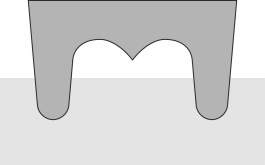
To account for the added mass, we need only modify one of the terms in the equation of motion. This means altering the quantity \(M\) that stands for the ship’s mass on the right-hand side of equation 1. For any given hull shape, the added mass is equal to a constant times the mass of the water deflected [15], and the value of the constant depends on the hull geometry. For the wall-sided vessel Cecily mentioned earlier, the problem is straightforward. The total volume of water deflected by the hull is equal to the hull’s own displacement, so in equation 1 we simply replace \(M\) by \(2M\), and similarly for equation 3, so that the period increases from 6.3 to 9.0 s, the same result we got when doubling the size of the hull with added mass ignored. However, the added mass varies also according to the type of motion under investigation. When a ship pitches, the calculation is more difficult. It’s difficult for rolling motions too, except that rolling motions tend to cause much less disturbance in the surrounding water, and if the cross-section of a ship is rounded in form as shown in figure 6, the disturbance may be sufficiently small for the added mass to be ignored.
Figure 6
The second difference has to do with damping. Damping is a general term for a process that inhibits oscillations by draining energy from the system, typically through friction. It is the function carried out by dampers (otherwise known as ‘shock absorbers’) that are fitted to an automobile suspension. They exert a resistance that is related to the speed of oscillation, and stop the vehicle from bouncing up and down repeatedly after hitting a pothole in the road. They also reduce the response to a regular series of bumps having the same frequency as the springs. Ships don’t have dampers; instead, they rely on the water, which resists oscillating motion in the same way that it resists the forward progress of the ship. The resistance is experienced as a change in the distribution of normal pressure over the hull surface together with viscous friction (there is a more rigorous explanation of the mechanisms involved in [16]). You can observe the effect yourself if you plunge your fist into a bowl of water and move it up and down. Waves will appear on the surface, carrying energy away from the centre of the disturbance, a visible sign of the damping effect that the water is exerting on your arm. To account for damping, one must introduce a new term into the equation of motion, because the damping force is a function of the ship’s velocity, which doesn’t appear in equation 1. However, at this point we’ll leave the question of heaving motions aside and turn to rolling motions instead.
Equation of motion in roll
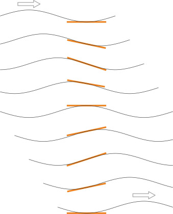
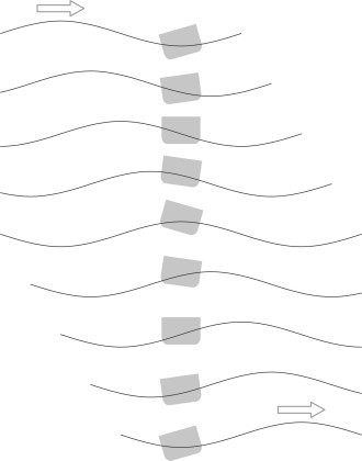
Roll is potentially the most dangerous of all the ship’s motions. In what follows we’ll write down the equation of motion and solve it to determine an expression for angle of roll produced by a sub-surface wave of known amplitude. Figure 7 shows the wave profile of a beam sea at successive moments in time, laid out in sequence from top to bottom of the diagram. The ‘input’ here is not the elevation of the water surface, but its slope \(\alpha\). In Appendix 2 we show that when a ship floating in still water rolls through a small angle, the centre of buoyancy moves in such a way as to generate a righting moment that is proportional to that angle. The question now arises what happens when the water surface itself is moving. We assume that the righting moment is unchanged, provided we base the righting moment on the angular deflection \(\phi - \alpha\) relative to the sloping surface. However, there is a complication. The hull doesn’t ‘feel’ the same pressures below the waterline as it would when rolling in still water, because the fluctuations in water pressure underneath a wave train decay with depth. As explained in Section M1820, at the depth of a ship’s keel, the motion of the water particles is reduced – specifically, the amplitude of the wave profile is less than the amplitude at the surface. We must compensate somehow for the attenuation, and a neat trick is to base the calculations not on the angle of the wave surface, but on the angle \(\alpha\) of the subsurface wave profile that passes through the ship’s centre of buoyancy. This was the method used by Froude in his early work on ship motions during the 19th century.
Figure 7
We can now write down the equation of motion and solve it to find an expression for the roll amplitude. Essentially, the equation embodies Newton’s Second Law applied to a rotating body, and its derivation is explained in Appendix 3. It is expressed in terms of couples and angular displacements rather than forces and linear distances, and it contains three terms:
(10)
\[\begin{equation} -C\frac{d \phi}{d t} - \rho g \nabla \overline{\text{MG}} (\phi - \alpha) \quad = \quad I_{xx} \frac{d^{2} \phi}{dt^2} \end{equation}\]The two terms on the left represent the two couples acting on the hull, the first being the damping couple, in which the quantity \(C\) represents a damping constant. The second term is the righting couple, the equivalent of the restoring force in heaving motion. Here, \(\overline{\text{MG}}\) refers to the metacentric height, and \(\alpha\) is the angle of the subsurface wave passing through the ship’s centre of mass. The term on the right is the equivalent of the ‘mass times acceleration’ term on the right-hand side of equation 1 for heaving motion, except that we’ve replaced the ‘mass’ by \(I_{xx}\), the rolling moment of inertia, and the angular displacement \(\phi\) for the linear deflection \(z\) throughout. In Appendix 3, we show that the roll angle relative to the water surface follows the harmonic curve given by
(11)
\[\begin{equation} \phi \quad = \quad \frac{ \alpha_0 }{ \sqrt{ \left[ 1 - \left( \frac{\Omega} {\omega} \right)^{2} \right]^{2} + 4 \zeta^{2} \left( \frac{\Omega}{\omega} \right)^{2} } } \cos \left( \Omega t - \delta \right) \end{equation}\]in which \(t\) represents time, \(\alpha_0\) is the amplitude of the wave slope, \(\zeta\) is known as the damping coefficient, \(\delta\) is the phase difference between the wave angle and the ship’s angle of roll, \(\Omega\) is the wave frequency, and \(\omega\) is the natural frequency of roll. Both \(\Omega\) and \(\omega\) are angular frequencies measured in radians per unit time.
Gain, resonance, and phase lag
The right-hand side of equation 11 tells us that the amplitude of the roll angle \(\phi\) is equal to the amplitude \(\alpha_0\) of the wave slope multiplied by a constant. The ratio of the two amplitudes is
(12)
\[\begin{equation} \frac{1}{ \sqrt{ \left[ 1- \left( \frac{\Omega}{\omega} \right)^{2} \right]^{2} + 4 \zeta^{2} \left( \frac{\Omega}{\omega} \right)^2 }} \end{equation}\]which in the language of signal processing is call the gain factor (or just gain). The derivation appears in Appendix 3. There are two key elements in this expression. The first is the quantity \(\Omega / \omega\). The black curve in figure 8 shows the gain factor plotted as a function of \(\Omega / \omega\) for a particular hull. The curve has the same form as the one used in Figure 6 of Section G1115 to represent the behaviour of a car suspension. The most prominent feature is the peak in the middle, which occurs when \(\Omega/\omega = 1\), the point where the wave frequency and the roll frequency coincide. Among other things, it divides the ship’s response into two distinct regimes. They arise because the rolling motion of a ship is out of step with the motion of the waves, and the phase difference is encapsulated by the phase angle \(\delta\), for which an expression is derived in Appendix 3. When \(\Omega/\omega\) is less than 1, meaning that the wave frequency \(\Omega\) is less than the ship’s natural frequency \(\omega\), the phase angle is negative and the ship motion leads: in nautical parlance, it ‘rolls away from the waves’. When \(\Omega\) is greater than \(\omega\), the phase angle is positive and the ship motion lags behind. Effectively, the hull ‘rolls into the waves’ as shown in figure 9 [20].
Figure 8
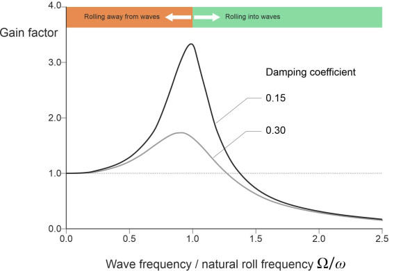
Figure 9
Ultimately, it is the height of the curve that measures the severity of the ship’s rolling motion. If the gain is greater than 1, the ship rolls through a greater angle than the water, in other words it amplifies the input, which of course is undesirable. On the other hand, if the gain less than 1, the ship rolls through a smaller angle, and effectively smooths out the wave input. This second result is the one we want. You can see that for very small frequencies (long wave periods) the ship is effectively ‘glued’ at right-angles to the wave surface: it rolls with the same amplitude as the wave and the gain is unity. There is no ‘magnification’. For very large frequencies (short wave periods), the ship is unaffected by the waves and doesn’t roll at all. The gain is zero.
Danger lurks in the area between. The roll amplitude rises to a peak at \(\Omega/\omega = 1\), where the wave period coincides with the natural period of roll. Here, the ship goes into resonance and according to equation 12, the value of the gain factor becomes \(1/2\zeta\). At this point, if there is no damping, \(\zeta\) is zero, so in theory, the gain is infinite and the oscillations run out of control. However, damping comes to the rescue. Its effect is to smooth out the motion in the same way that it smooths the ride of an automobile, by inhibiting the violent motions that would otherwise accompany resonance. In practice, there is always some degree of damping in the system, which arises naturally from friction or from fluid turbulence. Nevertheless, the gain factor for a conventional monohull can exceed 10 [14], meaning that a wave whose slope varies through the range \(\pm 1^\circ\) can make the ship roll through \(\pm 10^\circ\). The black curve in figure 8 was plotted assuming a damping coefficient of 0.15. By comparison, the grey curve shows the effect of raising its value to 0.3: the gain factor becomes less pronounced in the region of the resonant frequency. Improvements of this order can be achieved with various devices, for example bilge keels. These are strips of wood or metal running along the hull surface that project into the fluid and create friction that inhibits extreme rolling motions.
Before moving on, we might ask whether a similar phenomenon arises with heaving or pitching movements. The answer is that they both involve much larger added mass and damping forces, so for almost any shape of hull, the amplitude of heaving and pitching movements tends to peak at a relatively modest level, and therefore resonance seems to be less of a problem [17] [20] [14]. It is possible, however, to make a slender cylindrical body similar to a buoy, that floats with its axis perpendicular to the mean water surface. Its added mass is very small so that it heaves up and down in spectacular fashion when tuned to local wave conditions. Such devices have been proposed as a basis for generating electrical power from wave energy.
Composite motions
Earlier we examined the heaving motions and pitching motions of ship as two separate phenomena. But these motions rarely happen in isolation. When a ship rises over a wave crest, it moves bodily upwards and pitches aft at the same time. As it heads into the trough on the other side, it moves bodily downwards and pitches forward too. The motions are inter-linked, or in mathematical terms, coupled. They’re not the only motions that behave in this way: roll is coupled with heave too, because it’s driven by changes in the slope of the water surface as each wave passes across the ship’s path, and there must be a periodic rise and fall in the water level for this to happen – the ship heaves as it rolls. But in practice, one can treat the two motions as if they were independent, and predict the roll angle without explicitly modelling heave. By comparison, modelling the coupled pitch-and-heave combination is technically more difficult.
Pitch with heave
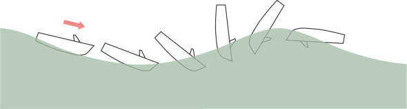
When a ship pitches, a new factor comes into play: the length of the waves. Let’s assume that the vessel is moving forward into a head sea. Waves that are appreciably shorter than the hull won’t make it pitch even if their period coincides with the natural period, because the hull bridges over them. The situation changes when the wavelength approaches the length of the hull. Now, the vessel will undergo heave and pitch together – it can straddle a wave crest with the bow and stern raised out of the water, meaning that the propeller is partly exposed, the engines race, and the vessel loses power (figure 10). Having passed over the crest it will surge down the far side and may ‘dive’ into the next wave, burying the bow under a wall of water (figure 11). During a ‘dive’, smaller boats have been known to ‘pitchpole’ as shown in figure 12; the boat’s momentum causes it to tumble end-over-end [1].
Figure 10
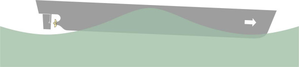
Figure 11
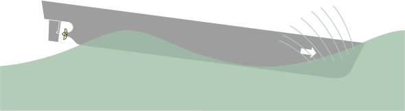
Figure 12
Now let’s turn the situation around and imagine the same waves arriving from the stern. Things may get worse, because in a stern sea, the wave encounter period increases and resonance becomes more likely. Also, vessels are less well equipped to handle waves arriving from the stern, which is wider than the bow and can be overwhelmed by a wave that breaks over the deck, in which case the ship is said to be ‘pooped’ (figure 13). Finally, the water particles in each wave crest are moving in the same direction as the ship, and when the peak of a particularly large wave passes underneath the stern, they may be moving faster than the ship itself. If so, the rudder is effectively moving backwards through the water, which reverses the normal steering action. It may be exposed as well. Either way, helm control is compromised at a critical moment.
Figure 13

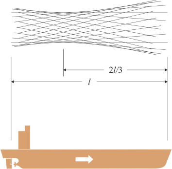
If it were possible for a ship to move up and down in a ‘pure’ heaving motion, all parts would be rising and falling together. By contrast, in a ‘pure’ pitching motion, the ship would rock back and forth, pivoting around a point roughly amidships, where the vertical motion would be zero. But since the motions are coupled, passengers and crew experience vertical oscillation at all points along the deck, with a larger amplitude at the bow and stern and a minimum somewhere in between. For most ships the minimum occurs at a point roughly 2/3 of the ship’s length from the bow [9] - if you are building a passenger liner, this might be a good place to put the restaurant. The motions are shown in figure 14 for a ship in sinusoidal waves of length equal to 2.5 times the hull length, assuming that the hull remains parallel to the wave surface throughout. Presumably, a similar phenomenon occurs with the corresponding movements in the horizontal plane, i.e., yaw and sway. I haven’t been able to find any data on this, but one source records that the minimum lateral movement observed on a particular ship occurred close to the bow [9]. This might be a good place to put the ballroom.
Figure 14
Parametric roll
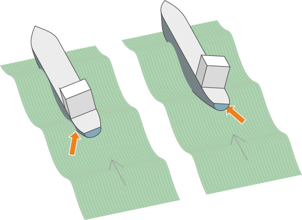
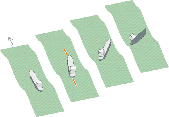
More serious is a form of composite motion that has emerged recently among container ships. When the vessel is heading straight into the waves, theory suggests it should heave and pitch without rolling at all. But under certain circumstances, the vessel may start rolling with an amplitude sufficiently large to shake loose the containers and threaten a capsize. The phenomenon is called parametric roll. It is usually explained as a consequence of two circumstances: (i) container ships tend to have a large bow flare and stern overhang, and (ii) the roll characteristics change as a wave crest moves along the hull because the cross-section changes: hence the overall righting lever undergoes a cyclic variation that can cause problems when the interval between successive wave crests roughly equals \(T_{R}/2\), one half the natural period of roll. The details are somewhat convoluted but we can explain the phenomenon in a simple way. Any perturbation – however small - that causes the hull to roll slightly to starboard say, will destroy the lateral symmetry, so when a wave encounters the bow flare, it will deliver a restoring impulse on the starboard side as shown in figure 15. The hull will then roll to port, where the bow flare encounters the next wave crest. A train of waves will deliver a regular series of pulses. If the encounter period is close to \(T_{R}/2\) and the ship continues to steer into the waves, the hull will begin to resonate and roll appreciably from side to side. Resonance of this kind can also happen in a following sea, particularly for ships with a flat transom stern where the wave crests can deliver upward impulses alternately on the port and starboard quarter as shown in figure 16 [8].
Figure 15
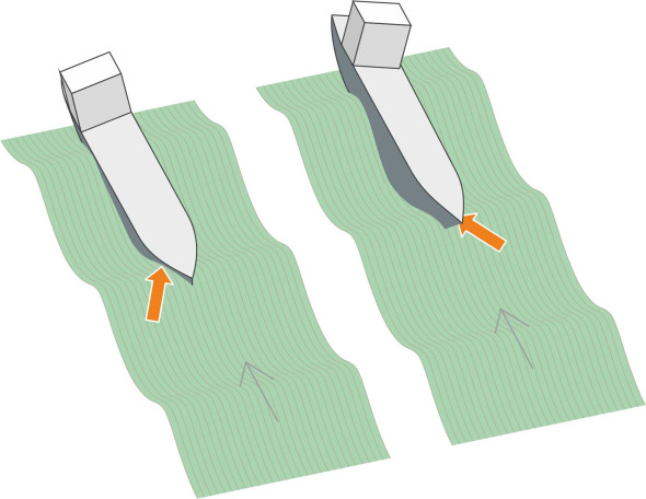
Figure 16
Broach
Last is a phenomenon that can threaten any ship when the waves arrive from astern: the broach. It has been the ruin of many sailing vessels. Normally, in stormy conditions a ship’s master will turn into the waves, but a sailing vessel can’t do this because it needs the power of the wind to maintain way so that the rudder works and the ship can be kept under control. In extreme conditions the crew can take in almost all the sails and let the ship run ‘before the wind’. But if it doesn’t keep up a certain speed, it is liable to broach and capsize. Figure 17 shows how the vessel falls broadside into a trough after a loss of control that builds up over several successive waves. The sequence is broadly as follows:
- A wave lifts the stern from behind, propelling it forward because the water in the crest is moving faster than the ship. At the same time, the bow plunges into the trough ahead, where the water is moving more slowly than the ship and resists the motion.
- The vessel is now in the grip of two opposing forces: one thrusting the vessel forward at the stern and the other holding the bow back. If the hull is not perfectly aligned in the direction of motion of the waves, the two forces will apply a couple that increases the yaw. For example if it is pointing to starboard, the wave makes vessel yaw more sharply to starboard.
- The helmsman tries to correct the yaw, but rudder adjustments in a large ship can take several seconds, and because the wave crest is moving faster than the ship, rudder control is temporarily reversed or has no effect at all. The hull continues to yaw until it is almost broadside on to the waves.
- Subsequent waves arrive on the ship’s beam. Their impact makes it roll severely, and may damage the steering gear and superstructure as they break over the gunwale. In a heavy sea, the vessel will take on water and eventually become overwhelmed.
Figure 17
Engineering for stability
Over the years, maritime nations have developed codes of practice intended to prevent unstable ships putting to sea, many of which are now incorporated into a unified framework under the aegis of the International Maritime Organisation (IMO). It is not easy to establish a minimum standard for ‘stability’ – in itself a complex notion - given the range of sea conditions and loading conditions that a vessel will face during its working life. Hence the international codes tend to focus on numerical indicators that are relatively easy to calculate and verify. For example, there are regulations intended to prevent the ship from rolling dangerously, and they are framed in terms of the righting lever together with the energy required to overcome the righting torque over roll angles up to \(40^\circ\) [18]. These are proxies for stability. They don’t tell you much about the ship’s behaviour in different circumstances, but they can be estimated from the drawings before construction begins, and therefore provide a safety net together with a consistent basis for regulatory control.
To meet the safety requirements and to present passengers and cargo with an acceptable degree of comfort, designers try to avoid resonance in any of the ship’s motions, and so prevent the hull from oscillating wildly under the action of waves. In particular, the natural period of roll shouldn’t fall within the spectrum of surface waves that the vessel encounters in normal service. The problem is that the sea produces waves of widely differing periods, ranging from a second or two in choppy water up to 20 seconds and beyond for large waves in a storm. So one tries to make the natural period of oscillation as long as possible: the longer the period, the less often the vessel will meet waves that are tuned to the same frequency.
Analysing the ship’s behaviour
If you are building a ship, you’ll want to know in advance how it will perform. Predicting a ship’s behaviour is a complex and expensive process. There are several ways of going about it. The first option is to build a prototype, send it out into the biggest storm you can find, and see what happens. The second is to make a miniature version of the ship and test it in a wave tank. Thirdly, you can analyse the motions and try to express them in the form of mathematical equations. Finally, you might attempt a computer simulation. All bar the first involve constructing a ‘model’ for the real thing - either a physical model or an abstract representation – and to keep the problem manageable, the model will embody a simplified representation of reality. Many models share the same simplifying assumptions, and it’s worth listing the most common ones. They are:
- The ship is rigid.
- There may be several different trains of waves arriving at the ship from different directions, but each wave-train is linear (i.e., sinusoidal).
- The ship’s response to each wave train is ‘linear’ too, in the sense that it is independent of the effects of any other wave train, and the combined effect is equal to the sum of the individual responses.
- The vessel is stable, so that it doesn’t undergo an extreme motion in response to a small input, as might happen for example if it were on the verge of capsizing.
- The viscosity of water is negligible except when modelling roll.
Finally, the simpler models assume a one-way interaction: approaching waves are not affected by the presence of the hull. This assumption is known as the Froude-Krylov hypothesis after two distinguished hydrodynamicists, William Froude and Alexei Krylov, both of whom used it as a stepping stone to analysing ship motions.
So far we have considered the motions heave, pitch and roll in isolation. But in a real seaway, to a greater or lesser degree all the motions happen at once. The ship will encounter waves of different frequency and height all arriving at the same time, and possibly from more than one direction. Somehow the model has to deal with the simultaneous ‘inputs’ and piece together their effects on the ship’s behaviour – the ‘output’. It helps if the individual wave trains are not too severe, so we can picture them as sine waves, each of which stimulates a forced simple harmonic motion response. Models of this type tend to be structured in a similar way. Following [3] and [12], we can sketch the steps in outline.
- Step 1: Represent the water surface as a superposition of harmonic waves of different frequencies (Fourier decomposition). These waves constitute the model ‘input’.
- Step 2: Solve the equations of motion to find out how the ship responds to each input frequency.
- Step 3: Express the results in the form of Response Amplitude Operator (RAO) values that describe for each frequency how the output (amplitude and phase of oscillation) is related to the amplitude of the wave input. Together, the RAOs define what is known in other fields as the frequency response function.
- Step 4: Use the RAOs to calculate the ship’s responses. The response at any particular frequency will depend only on the input together with the system characteristics at that frequency.
- Step 5: Superpose the responses to produce the overall output: the effects are additive except for the resistance, which is non-linear.
The computations required are expensive and time-consuming. Sea waves are considered to act on the vessel in the same way that a bumpy road surface acts on the suspension of an automobile, except that they impact whole length of the hull rather than just four wheels, and Step 2 is the biggest single challenge. In order to simplify Step 2, investigators have in the past divided the hull into short transverse segments or ‘strips’ with the forces and couples acting on each strip quantified separately. This is the basis of the ‘strip method’ often referred to in the textbooks [4] [13]. The repetitive nature of the process lends itself to computer analysis, using a software package to analyse the strips separately and combine the results. To improve realism, the equations can be embedded within a statistical framework that takes into account the irregularity of real waves, so the results can be expressed in terms of probabilities. However, techniques have changed in recent years with the arrival of CFD (Computational Fluid Dynamics) packages that speed up the whole process and yield more reliable results. They treat the water in which the ship is moving as if it were composed of small parcels, and track the movements of each parcel individually together with its impact on the hull.
So which of these approaches works best? Computer simulation works for a variety of hull shapes [2], and is the only choice for extreme situations where the response in non-linear, for example when a ship is close to capsizing. However, the results don’t always help the investigator to understand why the hull behaves as it does, or how to improve its performance. They have to be taken on trust, and different conditions explored by re-running the software each time. This is one reason why text books tend to focus on mathematical models. It’s true that mathematical equations describe a simplified version of reality otherwise they would be impossible to formulate, but a good model can throw light on what is going on even if it can’t give you a numerical forecast. For example, it might reveal that some parameters are more important than others, and tell us how they affect stability. It might also warn us if the design is flawed, and if so, what to do about it (for example, if the metacentre lies below the centre of mass the ship is almost certain to capsize, so lowering the centre of mass might be a good idea).
Hull shape
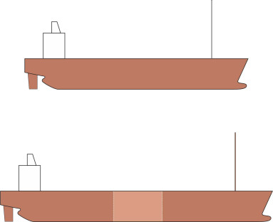
For longitudinal stability, a ship’s best protection is brute size: specifically, a long hull will bridge across most of the waves with less risk of slamming, diving and propeller exposure. Hence in rough waters it will not only be safer but it will have a speed advantage over a shorter vessel of equivalent capacity. This is why some owners will pay to have their vessels ‘stretched’ by adding new sections – not only will they carry more cargo, but they’ll carry it faster (figure 18 ). In addition, most ships nowadays have flared stems that resist being pushed below the surface. A bulbous bow is also thought to dampen pitch by providing buoyancy at the forward end. At wavelengths equal to the ship’s length or more, resonance in heave and pitch becomes likely [17], in which case the rise and fall of the bow will produce sharp impacts on the ship’s bottom underneath the stem. The phenomenon is called ‘slamming’, and we’ll return to it later in Section M1015.
Figure 18
Nevertheless, we hinted earlier that the most pressing requirement for any ship is stability in roll. There are three factors to consider. They are (a) the righting lever, (b) the natural roll period, and (c) the level of damping. Factor (a) we covered earlier in Section M1818, where it became clear that a ship with a high metacentre will strongly resist being overturned: the righting lever will cause it to rotate sharply back into an upright position when disturbed. This is a characteristic of boats with a shallow hull having a flat bottom and a wide beam like a punt for example: a wide hull is laterally more stable than other forms.
However, consideration of factor (b), the natural roll period, suggests that a wide beam isn’t necessarily an advantage in rough water. A wide beam means a shorter natural roll period, which exposes the ship to resonance. In relatively small waves, it will rock abruptly from side to side as it follows the jagged profile of the water surface. The high levels of acceleration entail:
- higher stresses in the hull,
- the possibility of shifting cargo, and
- difficulties for the crew, who may not be able to stand upright or do their job safely and consistently in a storm.
Mariners describe such a vessel as stiff, rather like a lorry equipped with stiff springs and a hard suspension. By contrast, a narrow hull has a lower metacentre and rolls at a lower frequency with less severe accelerations. Consequently its heeling motions are less severe, and in most conditions they lag behind the motion of the waves. Such a ship is described as tender, presumably because it imposes less severe loads and stresses on the hull and its contents. Also, resonance will occur less often because in good weather, the waves are small and their periods relatively short. Hence it makes sense to aim for a high natural roll period, which means keeping the metacentric height low. We already know from Appendix 2 in Section M1818 that the height of the metacentre increases with increasing beam so in principle we can improve matters by reducing the beam and increasing the draft. The trick is not to go too far and compromise static stability; the natural roll period for merchant ships is usually in the range 10 – 15 s, with passenger vessels towards the higher end of the range and cargo vessels towards the lower end.
Anti-roll measures
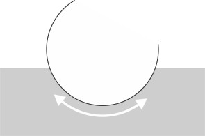
The third and final consideration relates to damping. A conventional hull relies mostly on friction to damp down rolling motions, as one can see by imagining a hull with a circular cross-section below the waterline as shown earlier in figure 6. When it rotates, it barely disturbs the surrounding fluid and doesn’t dissipate energy by creating waves, which leaves only viscous friction to slow it down. In reality, few ships are circular, but rather rectangular with rounded corners, but the damping effect is still small. Today, there are several devices that marine architects can install to damp down roll without making radical changes to the hull cross-section. They include
- bilge keels
- active fins
- passive anti-roll tanks
- passive or active moving weight systems.
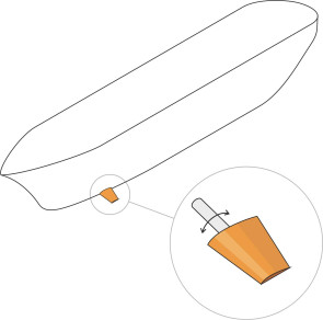
Bilge keels have been around for several centuries – we met them earlier in this Section and also in Section M1508. More recently, active devices such as moving fins, moving weights, and anti-roll tanks have been tried, of which the moving fins are the most common (see figure 19); they are fitted in pairs, one either side either near the bow or near the stern. The passive anti-roll tank is a clever device. Two tanks are fitted to the vessel, one on the port side and one on the starboard side, the two being connected by a pipe. They are partly filled with ballast fluid and the system as a whole is tuned to the natural roll frequency of the ship so that it damps the rolling motion at the most vulnerable frequencies. The principle is closely related to the tuned mass dampers commonly used to prevent tall buildings from oscillating in the wind, and there are other applications in the field of automobile engineering.
Figure 19
Postscript
On 18 December 1944, US Navy Task Force 38, a ninety-strong carrier fleet, was sailing across the Pacific Ocean. Its purpose was to conduct raids against Japanese airfields, and the ships were being refuelled in mid-voyage from the oil tankers that accompanied them. They knew they were sailing into bad weather, possibly a a typhoon. But the details were sketchy, and it was decided to continue the operation. As the wind rose to 160 km/h, the waves grew in size and some of the vessels lost contact with their neighbours. One by one they began to roll heavily and lose control, shipping water through the funnels and ventilators. It is hard to describe the resulting catastrophe. During a long struggle, three destroyers capsized and sank with the loss of 790 lives, while 9 other ships were damaged and over 100 aircraft were wrecked or washed overboard. The facts are set out in the web site [21] listed at the end of this Section, and there are many dramatic accounts elsewhere in the literature.
One hardly needs reminding that the sea is a potentially dangerous environment. But the warships of Task Force 38 had been designed to survive poor sea conditions, and what happened to them underlines how easily events can get out of control in bad weather. The sea surface is an interface between two fluids, and it generates waves that carry sufficient energy to damage or overturn a vessel weighing a hundred thousand tonnes.
Since 1944, the seakeeping performance of naval vessels and commercial ships has improved, although no-one has yet built a ship that is guaranteed to survive the most extreme storm conditions, partly because we don’t know what the most extreme conditions might be. The waves that do the most damage are random phenomena, with occasional ‘rogues’ that form when smaller waves pool their energy in ways that are not yet understood. Fortunately, with the help of satellite technology, meteorologists can forecast the conditions in which extreme waves are likely to occur with sufficient accuracy for mariners to avoid them. In the next Section we’ll try to visualise the impact that less extreme waves have on the ship’s hull.
Appendix 1: Heave in still water with no damping
We’ll assume that our ship has vertical sides above and below the design waterplane, and that it is floating in still water. Imagine that momentarily, it is forced downwards a little by some external agency. When released, it will rise again and continue to oscillate like a motor car on its springs. If the initial deflection is \(z\), it will displace an additional amount of water equal in volume to \(Az\) where \(A\) is the waterplane area. This produces restoring force \(F\) equal to \(- \rho g A z\) force units where \(\rho\) is the mass density of seawater. \(F\) is negative because it’s in the opposite direction to \(z\), and since it is proportional to the deflection, this is a case of simple harmonic motion. According to Newton’s Second Law, \(F\) equates to the product of the mass \(M\) of the floating body and its acceleration in the direction of \(z\). The equation of motion then becomes:
(13)
\[\begin{equation} M \frac{d^{2} z}{d t^2} \quad = \quad - \rho g A z \end{equation}\]or
(14)
\[\begin{equation} \frac{d^{2} z}{d t^2} + \frac{\rho g A z}{M} \quad = \quad 0 \end{equation}\]The general solution is:
(15)
\[\begin{equation} z \quad = \quad C_{1} \sin{ \omega t } + C_{2} \cos{ \omega t } \end{equation}\]where \(C_1\) and \(C_2\) are arbitrary constants that depend on the initial conditions [10] while
(16)
\[\begin{equation} \omega \quad = \quad \sqrt{ \frac{\rho g A }{ M } } \end{equation}\]The quantity \(\omega\) is the angular frequency expressed in radians per second, so the frequency \(f\) in cycles per second or Hz is given by
(17)
\[\begin{equation} f \quad = \quad \frac{1}{2 \pi} \sqrt{\frac{\rho g A }{ M } } \end{equation}\]and the period \(T_H\) in seconds by
(18)
\[\begin{equation} T_{H} \quad = \quad 2 \pi \sqrt{ \frac{M }{ \rho g A } } \end{equation}\]This result appears in [20] in a different notation.
Appendix 2: Roll and pitch in still water with no damping
We’ll begin with roll. Imagine that the ship is rotated momentarily by some external agency so it heels to one side by an angle \(\phi\), and is then released. In what follows, we’ll assume \(\phi\) is small and ignore the viscosity of the water, which exerts frictional resistance on the hull. We’ll also ignore added mass, which plays a relatively small part in roll. We already know from equation 9 in Section M1818 that when a ship rolls, the centre of buoyancy shifts transversely so that the line of action of the ship’s weight and the line of action of the buoyancy upthrust are separated by a horizontal distance known as the ‘righting lever’ \(r\) given by
(19)
\[\begin{equation} r \quad = \quad \overline{ \text{MG} }. \phi \end{equation}\]where \(\overline{ \text{MG} }\) is the metacentric height in roll. The ship’s mass produces a restoring couple about the centre of buoyancy. The ship’s mass equals the volume displacement \(\nabla\) times the density \(\rho\), so the restoring couple can be written as \(\rho g \nabla r\) , and if we substitute the right-hand side of equation 19 for \(r\), this becomes
(20)
\[\begin{equation} \text{ Restoring couple } \quad = \quad \rho g \nabla. \overline{ \text{MG} }.\phi \end{equation}\]Since the restoring couple is proportional to the angular deflection, we have another case of simple harmonic motion. As with the heaving problem, we now invoke Newton’s Second Law but this time in the context of angular motion, i.e., the product of the moment of inertia and angular acceleration in the direction of \(\phi\) will be equal to the applied couple, so that
(21)
\[\begin{equation} - \rho g \nabla .\overline{ \text{MG} }.\phi \quad = \quad I_{xx} \frac{d^{2} \phi}{dt^2} \end{equation}\]where \(I_{xx}\) is the moment of inertia of the ship around its longitudinal axis. This can be re-arranged to give
(22)
\[\begin{equation} \frac{d^{2} \phi }{d t^2} + \frac{ \rho g \nabla .\overline{ \text{MG} } }{I_{xx}}\phi \quad = \quad 0 \end{equation}\]for which the general solution is
(23)
\[\begin{equation} \phi \quad = \quad K_{1} \sin{ \omega t } + K_{2} \cos{ \omega t } \end{equation}\]where \(K_1\) and \(K_2\) are arbitrary constants that depend on the initial conditions while
(24)
\[\begin{equation} \omega \quad = \quad \sqrt{ \frac{ \rho g \nabla .\overline{ \text{MG}} }{ I_{xx} } } \end{equation}\]The quantity \(\omega\) is the angular frequency expressed in radians per second so the natural roll frequency \(f_R\) in cycles per second or Hz is given by
(25)
\[\begin{equation} f_{R} \quad = \quad \frac{1}{2 \pi} \sqrt{ \frac{ \rho g \nabla .\overline{ \text{MG}} }{ I_{xx} } } \end{equation}\]and the period \(T_R\) in seconds by
(26)
\[\begin{equation} T_{R} \quad = \quad 2 \pi \sqrt{ \frac{ I_{xx} }{ \rho g \nabla .\overline{ \text{MG}} } } \end{equation}\]This result appears in [20] in a different notation.
The analysis for pitch follows the same sequence, except that the rotational movement now takes place around a different axis. In equation 26 we replace the moment of inertia in roll \(I_{xx}\) by the moment of inertia in pitch \(I_{yy}\), and replace the distance \(\overline{ \text{MG} }\) of the roll metacentre above the centre of mass by the distance \(\overline{ \text{MG}_P}\) of the pitch metacentre above the centre of mass. The result is
(27)
\[\begin{equation} T_{P} \quad = \quad 2 \pi \sqrt{ \frac{ I_{yy} }{ \rho g \nabla .\overline{ \text{MG}_P} } } \end{equation}\]Appendix 3: Forced oscillations in roll
In Appendix 2 we recalled that for small rolling motions in calm water, the lever arm \(r\) between the weight of the ship and the opposing buoyancy force was proportional to the angle between the ship’s vertical axis and the water surface, in other words, the roll angle \(\phi\). Here, we introduce a new factor – there is a train of waves arriving on the ship’s beam that stimulates the rolling motion and controls the period of oscillation. The waves are sinusoidal with amplitude \(\alpha_0\). At any given instant, let the roll angle of the vessel be \(\phi\), and the subsurface wave slope \(\alpha\). The sloping subsurface changes the lever arm to a new value \(r^{\prime}\). We reason that \(r^{\prime}\) is proportional to the angle between the ship’s vertical axis and the subsurface wave passing through the centre of mass, which is \(\phi - \alpha\). Hence
(28)
\[\begin{equation} r^{\prime} \quad = \quad \overline{ \text{MG} } \left( \phi - \alpha \right) \end{equation}\]and the righting couple becomes \(- \rho g \nabla \overline{ \text{MG} } \left( \phi - \alpha \right)\) . We’ll assume there is also a damping couple equal to the rate of rotation times a constant \(C\). We may now invoke Newton’s Second Law in the context of rotational motion (moment of inertia times angular acceleration equals the applied couple) to get the equation of motion:
(29)
\[\begin{equation} I_{xx} \frac{ d^{2} \phi }{dt^2} \quad = \quad - C \frac{d \phi}{dt} - \rho g \nabla \overline{ \text{MG} } \left( \phi - \alpha \right) \end{equation}\]where \(I_{xx}\) is the rolling moment of inertia. This can be written
(30)
\[\begin{equation} \frac{ d^{2} \phi }{dt^2} + \frac{C}{I_{xx}} \frac{d \phi}{dt} + \frac{ \rho g \nabla \overline{ \text{MG} }}{I_{xx} }.\phi \quad = \quad \frac{ \rho g \nabla \overline{ \text{MG} } }{I_{xx} }.\alpha \end{equation}\]We’ll assume the subsurface wave train has constant frequency \(\Omega\), and put
(31)
\[\begin{equation} \omega^{2} \quad = \frac {\rho g \nabla \overline{ \text{MG} } }{I_{xx}} \end{equation}\]and
(32)
\[\begin{equation} \zeta \quad = \quad \frac{C}{ 2I_{xx} \omega } \end{equation}\]The ‘input’ is the wave slope \(\alpha\), which varies sinusoidally, lagging \(90^{\circ}\) behind the wave height, so we’ll put
(33)
\[\begin{equation} \alpha \quad = \quad \alpha_{0} \sin{ \left( \Omega t + \frac{\pi}{2} \right) } \quad = \quad \alpha_{0} \cos{ \left( \Omega t \right) } \end{equation}\]then equation 30 becomes
(34)
\[\begin{equation} \frac{ d^{2} \phi }{dt^2} + 2 \zeta \omega \frac{d \phi}{dt} + \omega^{2}\phi \quad = \omega^{2} \alpha_{0} \cos{ \left( \Omega t \right) } \end{equation}\]in which \(\omega\) is the natural period of roll and \(\zeta\) is known as the damping parameter. This is one of two standard equations of motion for forced oscillations that apply under different conditions. The first applies when the input takes the form of a displacement, as is the case when a car wheel is deflected up and down by the road surface (see equation 6 in Section G1115). The second applies when the input is a force, which is the case here. We seek the ‘particular integral’ \(A \sin{ \left( \Omega t \right) } + B \cos{ \left( \Omega t \right) }\) in which \(A\) and \(B\) are arbitrary constants. This is the part of the solution that describes the ship’s long-term behaviour after adjusting to the motion of the waves (see for example [10]). The result emerges as:
(35)
\[\begin{equation} \phi \quad = \quad \frac{ \alpha_0 }{ \sqrt{ \left[ 1 - \left( \frac{\Omega} {\omega} \right)^{2} \right]^{2} + 4 \zeta^{2} \left( \frac{\Omega}{\omega} \right)^{2} } } \cos \left( \Omega t - \delta \right) \end{equation}\]where \(\delta\) represents the phase difference between the input and output. The phase difference arises because the ship rolls with the same frequency \(\Omega\) as the sea waves, but with a different amplitude and out of step, i.e., with a time lag that depends on the level of damping. Its value is given by
(36)
\[\begin{equation} \delta \quad = \quad \arctan \left[ \frac{ 2 \zeta \left( \frac{ \Omega }{ \omega } \right) }{ 1 - \left( \frac{\Omega}{\omega} \right)^{2} } \right] \end{equation}\]while the amplitude \(\phi_{0}\) of the ship’s response is given by
(37)
\[\begin{equation} \phi_{0} \quad = \quad \frac{ \alpha_0 }{ \sqrt{ \left[ 1 - \left( \frac{\Omega} {\omega} \right)^{2} \right]^{2} + 4 \zeta^{2} \left( \frac{\Omega}{\omega} \right)^{2} } } \end{equation}\]and therefore the gain factor is equal to
(38)
\[\begin{equation} \frac{ 1 }{ \sqrt{ \left[ 1 - \left( \frac{\Omega} {\omega} \right)^{2} \right]^{2} + 4 \zeta^{2} \left( \frac{\Omega}{\omega} \right)^{2} } } \end{equation}\]Acknowledgement
Illustration on opening page: drawing of an American clipper ship from the children’s magazine Harper’s Young People, 3 February 1880, public domain, via the web site http://www.reusableart.com/sailing-ship-32.html (accessed 17 May 2021).