F.1817
Fluid forces
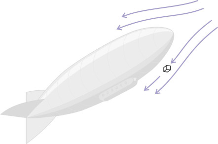
Occasionally when you’re outdoors on a windy day, a sudden gust will almost knock you over. The effect of the headwind on a saloon car is more powerful still. Together with the frictional shear stress, the pressure of the air flowing over the body surface will resist its motion, try to lift it off the ground, and maybe push it to one side as well. Where do these forces come from? Until recently, the mechanism wasn’t clear. Scientists once believed that ‘drag’ was caused by fluid particles striking the front of a moving body like grains of sand [9]. The idea was first promoted by Isaac Newton, and at the time, it made sense. But in the light of what we know today about fluid behaviour, the reality is more subtle. It’s true that in a gas, the molecules dart about and collide with rigid objects in their way, but their paths are not independent. Rather, they’re entangled like the fibres in cotton wool, and where their paths meet, the collisions between them amount to a form of collective behaviour. So a fluid – gas or liquid – behaves like a continuous and even slightly sticky substance, and when it encounters a moving body, its impact is modified by the forces acting among the particles themselves. Indeed, the internal forces arise from several distinct mechanisms all acting simultaneously. In this Section, we’ll try to understand how the mechanisms work, see how the internal forces change with the body’s speed and size, and sketch out a general formula for their impact on the moving body itself in terms of lift and drag.
Forces among the fluid particles
Let’s start by examining the forces from the fluid’s point of view. It helps to think of the vehicle as stationary while the fluid moves past it, and whenever a solid body interrupts their motion, fluid particles will divert around the perimeter, speeding up or slowing down during the process. A particle can’t change its velocity unless a force is applied to it, and since the forces vary from place to place within the flow field, its velocity \(U\) will vary from moment to moment while the speed \(V\) of the vehicle itself is fixed. It’s this mutual adjustment between the forces and accelerations in compliance with Newton’s Second Law that underpins the fundamental laws of fluid flow, in particular, the Navier-Stokes equations mentioned earlier in Section F1917.
Figure 1
Picture an imaginary rectangular box whose position is fixed relative to the vehicle, somewhere near the body surface as shown in figure 1, but not inside the boundary layer. Fluid particles flow through the box, which at any one time contains maybe a few billion molecules. Suppose its dimensions are \(\delta x\), \(\delta y\) and \(\delta z\). Since the sides of the box remain in fixed proportions, the physical scale of the element can be represented by a single yardstick. The yardstick we’ll use is the size of the vehicle itself, which we can represent by its overall length \(l\); in the picture we are about to describe, the value of \(l\) sets the physical scale not only of the vehicle but of all the ‘boxes’ in the flow field, so that together with the streamlines, their dimensions scale up and down in proportion to \(l\). Other important variables are the density of fluid \(\rho\), the coefficient of fluid viscosity \(\mu\), the acceleration due to gravity \(g\), and the speed of sound \(c\) in the fluid.
How the forces are produced
There are several ways in which the fluid in our box might interact with the wider world, through different types of force. The most important ones are:
- normal pressure,
- viscous shear force,
- gravitational force,
- elasticity, and
- inertia.
They divide into two categories: body forces and surface forces. In this context, a ‘body force’ is a force whose origins lie outside the flow field. It could be magnetic attraction for example, but the only body force we’ll need to consider here is gravitational pull, in other words the weight of the fluid contained in our particle. It acts vertically downwards, and it acts all the time regardless of what is happening elsewhere. The remainder are ‘surface forces’, all of which act at the interface with neighbouring particles. They manifest themselves through several distinct mechanisms that lie at the root of fluid behaviour and are accounted for in the Navier-Stokes equations. The equations are set out in the Appendix to Section F1917, which includes a Table showing how the forces map onto individual terms (note that there is no ‘elasticity’ term because in Section F1917 we assume the fluid is incompressible).
The five mechanisms produce internal forces of differing intensity, each scaling up and down with the size \(l\) and velocity \(V\) of the moving body in a distinctive way [16]. If we are designing a vehicle, say a Formula 1 racing car, we will need to know which mechanisms are important, which can be neglected, and how each of the forces varies with the speed of the car as it hurtles round the track. We’ll also want to know how they vary with the size of the vehicle. A formula that enables one to ‘scale’ the drag, say, from measurements on a model in a wind tunnel is a vital tool for engineers.
So let’s get down to it. On the assumption that the local velocity \(U\) of each particle scales up or down everywhere in proportion to the vehicle velocity \(V\), one can derive a formula showing how the magnitude of the force produced through each mechanism changes with \(V\), \(l\), and the other relevant parameters, and the results are set out in the right-hand column of table 1, with the inertia force in a separate row at the end.
| Force category | Underlying mechanism | Scales as |
|---|---|---|
| Pressure forces | Pressure gradient across the box | \(\Delta p l^2\) |
| Viscous forces | Viscous shear stress | \(\mu V l\) |
| Gravitational | ‘Static’ weight of fluid | \(\rho g l^3\) |
| Elastic | Compression: the fluid can contract or expand | \(\rho c^2 l^2\) |
| Inertial | Resultant force | \(\rho V^2 l^2\) |
In this Table, the quantity \(\Delta p\) represents the pressure difference between two opposite faces of the fluid element, while \(c\) is the speed of sound through the fluid, \(\mu\) is its dynamic viscosity, and \(\rho\) its mass density. How did we arrive at the expressions in the right-hand column?
The inertia force
We’ll begin with the inertial mechanism in the bottom line. In the textbooks you’ll normally find it at the top. We are treating it differently because the inertia force is not an independent force, but rather, the sum of all the others, a yardstick if you like by which to measure them. When a fluid particle moves across the flow field, it experiences forces at every moment along its path. They are the independent forces as listed in the first four rows of the Table, and they cause it to accelerate and decelerate (remember that a body travelling round a curve at constant speed is accelerating too, because the transverse component of its speed is continually rising; in effect, it is accelerating sideways). According to Newton’s Second Law, the sum of the applied forces acting in any given direction is equal to the mass of the particle \(m\) times its acceleration \(a\) in that direction. The quantity that analysts call the ‘inertia force’ is just the product \(ma\). So numerically, it is equal to the sum of the applied forces, and we can work out from Newton’s Law how it scales with the velocity of the fluid and the mass of the element. The argument is set out in Appendix 1. It turns out that the inertia force is proportional to \(\rho V^2 l^2\), which implies, for example, that if the speed of the vehicle doubles, the inertia force acting on each fluid particle will increase by a factor of 4. Similarly, if the speed remains unchanged but the vehicle (together with all the elements in the flow field) is scaled up to twice its original size, the inertia force acting on each element will again increase by a factor of 4.
The pressure force
Now let’s turn to the top of the list, where we find the two mechanisms that are responsible for propagating fluid forces from one particle to the next. The first is the pressure force. We’ve already seen in Section F1918 how the normal pressure varies from place to place in an ideal fluid flow around a cylinder: it’s high near the stagnation points and low where the streamlines curve around the flanks. Consider an individual fluid element. Box-shaped, it has six identical faces, and a normal pressure force acts on each face. If they were all equal, there would be no net force on the element and the pressure forces would play no part in its dynamic behaviour. What matters is the pressure gradient, a difference \(\Delta p\) between opposite faces that pushes the fluid in a particular direction. It is proportional to the cross-sectional area of the fluid element, which in turn is proportional to \(l^2\). Hence the fluid pressure force everywhere scales as \(\Delta p l^2\). If you double the size of the vehicle and all the elements, it will increase by a factor of 4. Note that the vehicle velocity \(V\) plays a role too, but it doesn’t appear explicitly in the formula: its effect is subsumed within the variable \(\Delta p\).
Viscous forces
Unlike pressure forces, viscous forces tend to be significant only within the boundary layer that clings to a moving body. As demonstrated in Section F1917, for a Newtonian fluid, the shear stress between opposite faces of a fluid element is equal to the dynamic viscosity \(\mu\) times the velocity gradient \(du/dy\) between the faces. The velocity gradient has units of speed divided by distance, so given that the fluid particle velocities everywhere in the flow field scale up or down in proportion to the vehicle velocity \(V\), the shear stresses acting on all the fluid elements will scale up or down in proportion to \(\mu V / l\). The shear force is equal to the shear stress times the cross-sectional area, and therefore the total shear force acting on our particle is proportional to \(\left( \mu V / l \right) \times l^2\), which equals \(\mu V l\). If the speed of the vehicle doubles, given geometrically similar scaling of the flow field, the shear force on each particle will increase by a factor of 2. If the size of the vehicle together with each element doubles, the shear force will again increase by a factor of 2.
At this point you may have spotted an apparent contradiction. We are saying here that shear forces scale up and down in proportion to \(\mu V l\), whereas in Section F1917, equation 14 tells us that the shear force acting on a flat plate aligned parallel to the flow is proportional to \(V^{9/5} b l^{4/5}\) where \(b\) is the width of the plate and \(l\) its length measured in the direction of flow - for geometrically similar scaling we can take \(b\) as proportional to \(l\) so this expression simplifies to \(V^{9/5} l^{9/5}\). Why the discrepancy? The reason is that the geometry of the boundary layer doesn’t scale with the size of the moving body in the way that we have assumed. For example, if you imagine the plate stretched so its length doubles to \(2 l\), the boundary layer doesn’t double in thickness everywhere along its surface. Between the leading edge and the halfway point at \(x = l\), in fact, it will remain unchanged. So while the viscous force mechanism does indeed scale as \(\mu V l\) throughout most of the flow field, what happens at the interface between the particles and the body surface is a different matter that we’ll pursue elsewhere.
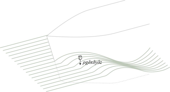
Gravitational forces
Gravitational forces are important for ships. A ship moving at a steady speed creates its own wave system that it carries along with the hull and this wave system accounts for a significant proportion of the total resistance. Let’s look more closely at a fluid element in the crest of one of the waves near the bow (figure 2). The weight of water in each wave crest presses downward and delivers a force equal to \(\rho g\) times its volume (\(\delta x . \delta y . \delta z\)) through its lower face onto the particle below. Since we take the particle dimensions as fixed in relation to the length of the ship it follows that the gravitational forces communicated through the fluid are proportional to \(\rho g l^3\), and they increase more quickly with our yardstick \(l\) than any of the other forces. When you double the scale of the vessel together with its surrounding flow field, the gravitational forces everywhere increase by a factor of 8. This assumes, however, that the wave height will rise and fall in proportion to \(l\), whereas in reality the wave height will also depend on how fast the ship is moving.
Figure 2
Elasticity forces
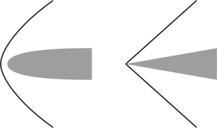
A high-speed aircraft can also generate waves, but waves of a different kind. As it approaches the speed of sound, a jet fighter (or any projectile such as a rifle bullet) creates shock waves that greatly increase the drag. At first sight, ships’ waves and supersonic shock waves appear to share a common structure, but in fact they are generated in different ways and have different geometrical shapes. The main difference is that a ship’s waves inhabit a different physical world: the interface between air and water. Water cannot easily be compressed, so when disturbed, it deforms by crossing the boundary to form crests and troughs in a regular pattern whose geometry doesn’t change when the ship changes speed. By contrast, air is ‘elastic’ – under pressure, it will squeeze into a smaller space, so that when travelling at high speed, an aircraft compresses the air particles ahead of its wings and fuselage into a narrow band or shock wave whose geometry varies according to the shape of the leading edge (figure 3). The air slows down as it passes through the shock wave, its density increases, and the pressure rises sharply from around 1 atmosphere to as much as 20 atmospheres [5] over a distance of the order of \(10^{-5}\) cm. Hence the shock wave is much thinner than a piece of paper [5]. At the same time, the temperature of the air particles rises as their kinetic energy is converted into heat. But here, we’re more interested in the forces that accompany the contraction. Picture a fluid element in the shape of a rectangular block having six faces, and choose any one of the faces. Suppose it has area \(\delta A\). As the fluid element passes through the shock wave, its volume shrinks by a proportion \(\alpha\), say. The pressure increase needed to bring this about is by definition \(\alpha E\) where \(E\) is the bulk modulus of the fluid. In turn this implies a force acting on the chosen face equal to \(\alpha E . \delta A\). It can be shown that for a perfect fluid the bulk modulus is equal to \(\rho c^2\) where \(c\) is the speed of sound in the fluid. On substituting for \(E\) we find the elastic force acting on our chosen face equals \(\alpha \rho c^2 . \delta A\), which is proportional to \(\rho c^2 l^2\).
Figure 3
Forces acting on the vehicle
To summarise, each fluid particle experiences a set of forces, one of which is a body force while the remainder arise from contact with neighbouring particles. The contact forces undergo a process of mutual adjustment, so that the particles move together in formation along streamlines that curve around the vehicle, some close to the vehicle body, and some further away.
What happens at the body surface
But the particles closest to the vehicle body surface act as a channel of communication, transmitting forces between the fluid mass and the vehicle. Within this ‘communication channel’, any distinction between the four fundamental force mechanisms at work in the fluid mass – pressure, viscous force, gravitational force, and elastic force - is lost. The vehicle ‘feels’ only (i) normal pressure, and (ii) shear stress. This doesn’t mean the fundamental mechanisms are unimportant, just that we’re not going to detect them individually by observing what happens to the vehicle. More to the point, we can’t predict what will happen to the vehicle just by adding the four forces together - having done all this work to establish how each force scales up or down with the vehicle’s size and speed, we are no closer to predicting how their overall impact will change. But as we’ll see shortly, the four forces help to explain at least qualitatively why different objects behave differently at different speeds, and in addition can be re-assembled into dimensionless parameters that form the building blocks for further analysis together with experimental measurements in towing tanks and wind tunnels. For the moment, we’ll picture them in combination as a single force, a vector at some angle to the direction of motion, which we’ll break it down into three orthogonal components: a component parallel to the longitudinal axis, a vertical component, and a transverse component. The longitudinal component, which opposes the motion, is ‘drag’. Of the other two, the vertical one is usually more important. It is called ‘lift’. The transverse component can make the vehicle difficult to control.
Estimating the forces
In reality, there’s no simple formula for predicting the overall drag, lift, or transverse force on a moving vehicle. This would mean solving the Navier-Stokes equations, which require the body shape to be described in mathematical terms. However, the body of a saloon car doesn’t conform to a mathematical formula, and even if it did, it would have to be a very simple one, because the Navier-Stokes equations have only a few known solutions, all of which apply to simple geometrical shapes. Hence fluid mechanics is an empirical science, and in practice, the designer will usually build a model and measure the forces on it directly, or simulate them on a computer. It helps if the shape of the vehicle, the speed of travel, and the fluid characteristics are all fixed in advance, in which case, a single experiment will provide useful information. However, there are many parameters involved, and the designer will usually want to try out variations in the body shape and vehicle performance over a range of operating conditions. There are many possible combinations of parameter values, and without a radical re-structuring of the problem, the workload can quickly get out of hand. The answer is to reduce the number of independent variables by bundling them together.
Dimensional analysis
Earlier in Section C1416 we quoted without much justification a formula for the air resistance experienced by an automobile. Here it is again, in a slightly different notation with the resistance denoted by \(D\) and the vehicle velocity by \(V\):
(1)
\[\begin{equation} \text{Drag or resistance } D \quad = \quad \frac{1}{2} \rho V^{2} A C_D \end{equation}\]where \(\rho\) is the density of air, \(A\) is the cross-sectional area of the vehicle body, and \(C_D\) is the drag coefficient. It’s a compact way of describing what fluid does to a moving body, and we shall try and figure out where the various terms come from and explain the all-important drag coefficient on the right-hand side. First let’s remind ourselves that each quantity that features in a physical law has attached to it one or more units of measurement. The quantity \(D\) is often measured in newtons, \(V\) in metres per second (m/s), \(A\) in square metres (m2), and \(\rho\) in kilograms per cubic metre (kg/m3). The drag coefficient is a ‘pure’ number having no units at all. For practical reasons, you would expect the units to be consistent throughout, so for example if \(V\) were measured in metres per second, then \(A\) would be measured in square metres and not square feet - otherwise, the numbers would get confused and the formula would deliver the wrong answer.
But there is a deeper principle at work here: a physical law must be true regardless of the units of measurement. This means that the ‘dimensions’ on either side of the equation must tally. The dimensions are not units as such, but categories of unit, principally mass, length and time denoted respectively by \(M\), \(L\) and \(T\). For example, speed is measured in terms of distance per unit time, which we can symbolise as \(L T^{-1}\). Area is measured in terms of distance squared, or \(L^2\). Let’s see how equation 1 looks if we replace the variables by their respective dimensions. Drag is a force, whose dimensions are those of mass (dimension \(M\)) times acceleration due to gravity (dimension \(L T^{-2}\)). Density has dimensions \(M L^{-3}\), speed has dimensions \(L T^{-1}\), and area has dimension \(L^2\). The drag coefficient has no dimension at all, so for the moment it can be left out of the analysis. Substituting these expressions in equation 1 we get
(2)
\[\begin{equation} M L T^{-2} \quad = \quad \left( M L^{-3} \right) \left( L T^{-1} \right)^2 \left( L^2 \right) \end{equation}\]and after tidying up the right-hand side by collecting like terms you’ll see that it comes to \(M L T^{-2}\) and therefore matches the left-hand side. Otherwise, something would be wrong.
How does this help? If you are trying to develop a formula for a physical quantity such as the total resistance acting on a ship you can use the dimensions attached to the variables to guide you towards an appropriate structure. The process involves a mixture of art and science, with some deep philosophical issues lurking in the background [23] [24]. Rather than go into depth, we’ll work out an example from first principles: a formula for the resistance of a ship. We start by trying to identify all the variables that might play a part. The ones that come to mind straight away are the ship’s speed \(V\) and its size. The ‘size’ of a vessel could in principle be represented by the waterline length \(l\), or the cross-sectional area, or the volume displacement. For a hull of any given shape, these last two are respectively proportional to \(l^2\) and \(l^3\) so in a sense the length, area, and displacement are all interchangeable. We shall also need the density \(\rho\) of the water in which it floats together with the kinematic viscosity \(\nu\). The mass of the ship is not required because it is effectively determined by the hull displacement and the density of water. Finally, we add the acceleration \(g\) due to gravity, which is an essential factor in the gravitational forces implicated in the ship’s wave system.
The next step is to express the result we want, the drag \(D\), as a function of some or all of the relevant variables. We then create a new set of variables to replace them, each having a dimensionless form. The power of dimensional analysis stems from the fact that by doing this, we effectively reduce the number of variables together with the range of possible formulae for the quantity we are trying to predict. Although it doesn’t give us a specific formula, it suggests a plausible structure and greatly reduces the number of experiments needed to determine the answers we want.
So let’s re-state the problem in more technical terms. Our task is to assemble the variables into dimensionless groups that are functionally independent - by ‘functionally independent’ we mean that none can be duplicated by combining the other terms in some way. Here, we are looking for distinct combinations of the variables \(D\), \(l\), \(\rho\), \(\nu\), \(V\), and \(g\). Each combination will be a multiple of one or more of the variables each raised to an arbitrary power. There are two ways of going about this. We shall use the simpler and more direct method, well over a hundred years old. It originated with John William Strutt, the third Baron Rayleigh. Lord Rayleigh worked in the field of sound and vibrations, and helped to establish a body of methods loosely known as ‘similarity principles’ that are widely used in fluid mechanics problems today. The working is set out in detail in Appendix 2. It yields a set of three groups: \(D / \left( \rho V^{2} l^{2} \right)\), \(V l / \nu\), and \(V / \sqrt{gl}\) [17]. The first is a dimensionless form of the resistance - it’s the quantity we are trying to predict. The other two can be pictured as independent variables that one can manipulate to increase or decrease the resistance. Assuming we have made the correct assumptions, they are the only quantities that matter in the sense that they summarise all the possible ways in which the variables we have identified can influence a ship’s resistance – we have effectively boiled down the number from five to two. Grouping the variables in this way means we don’t have to investigate the effects of changing \(l\), \(\rho\), \(\nu\) and \(V\) individually and therefore the number of combinations is drastically reduced. At a more general level, data becomes easier to interpret, and theoretical models easier to understand [20]. So our formula for a ship’s resistance is:
(3)
\[\begin{equation} \frac{D}{\rho V^{2} l^{2}} \quad = \quad f_{1} \left( \operatorname{Re}, \text{Fr} \right) \end{equation}\]in which the notation \(f_1 \left( . \right)\) stands for some unspecified function of Re and Fr. These two variables are the Reynolds number and the Froude number respectively. The Reynolds number was introduced earlier in Section F1917, and the Froude number features prominently in Section M1620 and M1619. They’re not just abstract numbers like the mathematical constant \(\pi\). They say something vital about the force mechanisms listed earlier in table 1. Take the Reynolds number first. It represents the ratio of inertial forces \(\rho V^{2} l^{2}\) to viscous forces \(\mu V l\), so that:
(4)
\[\begin{equation} \operatorname{Re} \quad = \quad \frac{\rho V^{2} l^{2}}{\mu V l} \quad = \quad \frac{ \rho V l}{ \mu } \quad \text{or} \quad \frac{Vl}{\nu } \end{equation}\]If Re is small (low speed, small vehicle), the viscous forces have a powerful influence on the fluid’s behaviour.
We can explain the Froude number in a similar way but we’ll square it first: the square of the Froude number is what you get if you divide the inertial force \(\rho V^2 l^2\) by the gravitational force \(\rho g l^3\) so that:
(5)
\[\begin{equation} \text{Fr}^{2} \quad = \quad \frac{\rho V^{2} l^{2}}{ \rho g l^{3}} \quad = \quad \frac{ V^2 }{ g l } \end{equation}\]For a slow-moving vessel, Fr is small, meaning that the gravitational forces have a more powerful influence than the viscous ones. And at any given speed, the gravitational forces increase with increasing vessel size: much of the engine power of an ocean liner is devoted to making waves. The Froude number can also be applied to other kinds of motion including, for example, animals walking and running, in which case the gravitational forces refer not to wave-making but the vertical oscillations of the animal torso that occur during each stride [10].
Although we won’t go into detail here, one can carry out a similar analysis for aircraft. The results are different, because unlike water, air is not a dense fluid and gravitational forces don’t play a significant role. So we won’t need the Froude number to appear on the right-hand side. Instead, the compressible nature of the fluid emerges as a significant factor especially at high speeds. So we compare the inertia force with the elastic force, and if we divide the inertia force \(\rho V^{2} l^{2}\) by the elastic force \(\rho c^{2} l^2\) we get the square of the Mach number, the Mach number being the ratio of the aircraft speed to the speed of sound:
(6)
\[\begin{equation} \text{Ma}^2 \quad = \quad \frac{\rho V^{2} l^{2}}{ \rho c^{2} l^{2}} \quad = \quad \frac{V^2}{c^2} \end{equation}\]This is the third in our trio of important dimensionless parameters. A high value tells us the elastic force is small. This doesn’t mean that compressibility effects can be ignored, quite the opposite. When the elasticity of the air diminishes it means that it can’t be compressed around the wings and fuselage quickly enough to get out of the way. As though hit with a hammer, it collapses into a shock wave, and the shock wave becomes a major contributor to drag. Turning back to equation 3, we can now get an equivalent formula for the resistance incurred by an aircraft if we replace the Froude number on the right-hand side with the Mach number Ma thus:
(7)
\[\begin{equation} \frac{D}{ \rho V^{2} l^{2} } \quad =\quad f_{2} \left( \operatorname{Re},\text{Ma} \right) \end{equation}\]where \(f_{2} (.)\) stands for another unspecified function.
Formulae for lift and drag
Our aim is to construct a formula that will enable us to predict the resistance incurred by a moving vehicle – any vehicle. We’ve already done it for ships, and the results appear in equation 3, in which the dimensionless parameters Re and Fr appear in place of the original variables \(l\), \(\rho\), \(\nu\), \(V\), and \(g\). A similar process gave us an equivalent result (equation 7) for aircraft. It’s a short step from here to a general formula that applies to all kinds of vehicle (land, sea and air). It only requires us to incorporate all three dimensionless variables into the expression on the right-hand side thus:
(8)
\[\begin{equation} \frac{D}{ \rho V^{2} l^{2} } \quad = \quad f_{3} \left( \text{Re, Fr, Ma} \right) \end{equation}\]It is usual to express equation 8 in a slightly different form. We’ll replace \(l^2\) by an equivalent surface area \(A\), multiply both sides by \(\rho V^{2} A\), and substitute ½\(C_{D}\)(Re, Fr, Ma) for the function \(f_3\)(.) on the right-hand side to get
(9)
\[\begin{equation} D \quad = \quad \frac{1}{2} \rho V^{2} A C_{D} \left( \text{Re, Fr, Ma} \right) \end{equation}\]which is the familiar drag equation we quoted earlier (equation 1). It has a distinctive mathematical structure, one that occurs across a whole range of problems in fluid mechanics, and it raises three questions: (i) why do the quantities \(\rho\), \(V^2\) and surface area \(A\) appear on the right-hand side in this particular arrangement, (ii) how does the formula tally with the different force mechanisms mentioned earlier, and (iii) what is the significance of the coefficient \(C_D\)?
The terms on the right hand side fall naturally into three groups like three pieces of a jigsaw puzzle, each with a distinct physical meaning. The first group is the expression ½\(\rho V^2\). It has units of force divided by area, and is identical to the ‘dynamic pressure’ term in the Bernoulli equation (see equation 24 in Section F1918; if you imagine a stream of particles hitting the body so they are brought to a halt and all their momentum dissipated, the body would experience a pressure or stress opposing its motion equal to ½\(\rho V^2\) per unit area). The second piece of the jigsaw puzzle is the term \(A\), which is a reference area denoting the ‘size’ of the body. It is natural to think of it as the surface area over which the dynamic pressure acts. How it maps onto the body surface depends on the nature of the resistance. If the resistance is largely due to pressure drag (i.e., it arises from a normal pressure difference between front and rear), the area that matters is the cross-sectional area measured perpendicular to the flow. If the resistance is dominated by shear forces, it will be the surface area measured parallel to the fluid flow, like the area of a yacht’s sail. If, as in most cases, the body generates both types of resistance, one can’t identify a specific region of the body surface over which the stresses act. However, we still need a reference area to help us determine how the drag for a body of any given shape varies with its physical size. In practice, for automobiles the reference area is usually the frontal area, while for an aircraft wing it is usually the plan area. For ships, it is the wetted area of hull.
Multiplying the dynamic pressure by the reference area gives us the quantity ½\(\rho V^{2} A\). It reminds one of the expression in table 1 for the inertial force, and it has the same units. You can think of it as a measure of the overall drag force - not the actual drag, but a notional value, the drag that would occur if the fluid particles impacted the reference area and stopped dead. But in reality the particles curve around the body profile and while some of them slow down, they don’t usually come to a halt, so the stresses they exert on the body surface are modified by its shape. The influence of body shape is represented by the third piece of the jigsaw puzzle, which is the drag coefficient \(C_D\). If \(C_D\) is less than 1, not all the energy of the fluid particles approaching the reference area is lost: a streamlined body will deflect them smoothly around the body contours and lessen their impact. On the other hand, a \(C_D\) value greater than 1 indicates that the fluid flow separates around the body perimeter to produce a wake whose diameter may be larger than the body itself. The expanded wake consists of ‘dead air’ or ‘dead water’ that constitutes an obstacle to the approaching fluid particles, as if the body had grown in size. Think of \(C_D\) as a magnification factor that scales up or down the retarding effect of the fluid on the reference area.
So the problem of estimating resistance boils down to finding the value of \(C_D\) . It is an unknown function of the three parameters Re, Fr and Ma, but depending on the kind of vehicle we are dealing with, not all three play a significant role. A passenger airliner doesn’t make waves on the sea so the Froude number can be omitted, leaving the drag coefficient as a function of Re and Ma only. The same applies to an automobile or a railway train, and since neither is likely to break the sound barrier we can omit Ma as well, leaving \(C_D\) as a function of Re only. In fact we can go a step further. Given a high Re and turbulent flow, the viscous effects are relatively small and the drag scales roughly with the inertial forces; in other words it’s proportional to \(\rho V^{2} l^{2}\). Looking at equation 9, you can see this implies that the drag coefficient is roughly constant [21]. For sharp-edged bodies in particular, \(C_D\) tends to be insensitive to Re because flow separation occurs at a fixed location on the body surface independently of flow conditions within the boundary layer. A constant drag coefficient is extremely useful: you only have to measure it once and the same value can be applied across a range of vehicle speeds. However, for streamlined bodies, \(C_D\) tends to fall in inverse proportion to the square root of Re [1].
Having worked out a general formula for the drag, we can follow a similar procedure to determine the lift \(L\), expressed in terms of the lift coefficient \(C_{L}\)(Re, Fr, Ma). Without going into detail, we’ll quote the result, which is:
(10)
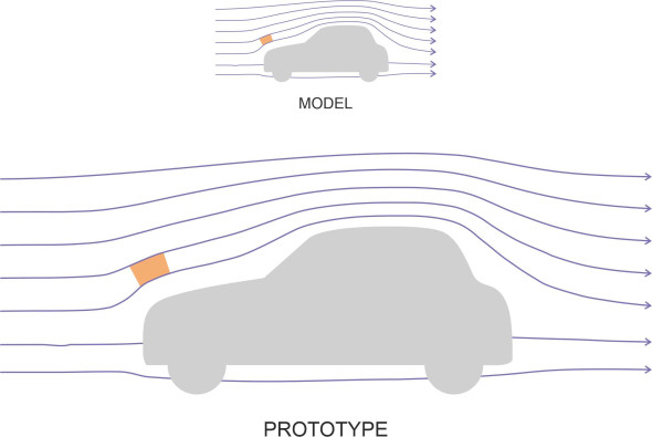
\[\begin{equation} L \quad = \quad \frac{1}{2} \rho V^{2} A C_{L} \left( \text{Re, Fr, Ma} \right) \end{equation}\]We can use equations equation 9 and equation 10 to estimate the drag and the lift for a moving body provided we know the values of \(C_D\) and \(C_L\) for a body of similar shape. There is no reliable method for determining their values from theory alone, but they can be estimated from experiments with a scale model in a wind tunnel or a water tank, and in principle the results will apply to the full-scale vehicle regardless of its size. In what follows, we’ll call the full-sized vehicle the ‘prototype’, and denote any quantity relating to to the prototype by the subscript \(p\), for example its velocity is written as \(V_p\). All quantities relating to the model will be denoted by the subscript \(m\).
Similarity and scaling rules
We have to set up the experiment so that the flow field around the model accurately represents the flow field around the prototype, i.e., that the model and prototype are ‘similar’ in a strict technical sense. There are three levels of similarity. At the bottom level, there is geometrical similarity: the model and prototype must have same shape, though not necessarily the same size. The ratios of all the dimensions of the model to the corresponding dimensions of the prototype must be the same. This includes the surrounding flow field, so that the geometry of the streamlines, the gaps between them, and the sizes of any fluid elements must scale up and down in the same ratio as the model length \(l\) (figure 4). At the next level comes kinematic similarity: the ratios of the velocities of all the particles in the model flow field to those of the corresponding particles in the the prototype flow field must be equal. At the third and highest level, dynamic similarity, the ratios of the fluid forces acting on the model to the corresponding forces acting on the full-size vehicle must all be the same. In fact, if this happens, the first two conditions will hold as well.
Figure 4
So how does the experimenter ensure that these conditions hold? You’ll recall that there are at least five distinct categories of force mechanism acting on each element in a flow field: pressure force, viscous shear stress, gravitational force, elastic force, and inertia. At first, the condition we are seeking appears to be impossible, because each force mechanism scales with the speed and size of the moving vehicle in a different way as specified in the last column of table 1. To guarantee dynamical similarity, we’ll have to manipulate the parameter values for the model test individually. Let’s take a simple example. Suppose our vehicle is an electric tram or trolleycar designed to cruise at 75 km/h; there are no wave-making forces and no elasticity forces so the only forces we need to consider are the inertia force and the viscous shear force. Denote the length of the model by \(l_m\), its velocity by \(V_m\), the viscous and inertia forces acting on the model by \({F_{m}}^{viscous}\) and \({F_{m}}^{inertia}\), and the density and viscosity of the fluid in which the model tests are carried out by \(\rho_m\) and \(\mu_{m}\) respectively. Also denote the corresponding values for the ‘prototype’ (the full-size vehicle) by \(l_p\), \(V_p\), \({F_p}^{viscous}\), \({F_{p}}^{inertia}\), \(\rho_p\) and \(\mu_p\). The condition we are trying to meet is that the viscous forces for model and prototype are in the same ratio as the inertia forces thus:
(11)
\[\begin{equation} \frac{{F_{m}}^{viscous}}{{F_{p}}^{viscous}} \quad = \quad \frac{{F_{m}}^{inertia}}{{F_{p}}^{inertia}} \end{equation}\]which we’ll re-arrange in the form
(12)
\[\begin{equation} \frac{{F_m}^{inertia}}{{F_m}^{viscous}} \quad = \quad \frac{{F_p}^{inertia}}{{F_p}^{viscous}} \end{equation}\]After substituting the appropriate expressions from the last column of table 1, this becomes
(13)
\[\begin{equation} \frac{\rho_{m} {V_m}^{2} {l_m}^{2}}{\mu_{m} V_{m} l_{m}} \quad = \quad \frac{\rho_{p} {V_p}^{2} {l_p}^{2}}{\mu_p V_p l_p} \end{equation}\]or, after simplifying,
(14)
\[\begin{equation} \frac{\rho_{m} V_{m} l_{m} }{\mu_{m}} \quad = \quad \frac{\rho_{p} V_{p} l_{p}}{ \mu_p} \end{equation}\]The expressions on the left-hand side and the right hand side are respectively the Reynolds numbers for the model and prototype, and the equation is saying that we’ll have dynamic similarity if the two are equal. We can see this from a different angle by looking at equation 9: if the Reynolds numbers are the same, then the drag coefficients of the model and prototype are the same. But what does this requirement entail for the model experiment? Assuming that the fluid used in the model test is the same fluid as the one in which the full-size vehicle operates, equation 14 simplifies to
(15)
\[\begin{equation} V_{m} l_{m} \quad = \quad V_{p} l_{p} \end{equation}\]In other words, we scale the speed of the fluid in the wind tunnel in inverse proportion to the length of the model. If the model is 1/5th scale with \(l_m\) equal to \(l_{p} /5\), the wind tunnel must operate at a fluid velocity 5 times the cruising speed for the prototype trolleycar, i.e., 375 km/h. It’s a tall order, but not impossible.
What about ships? Here, the problem is more complicated because the gravitational force mechanism comes into play as well, so we must add a new condition to equation 11: the gravitational forces for model and prototype must be in the same ratio as the inertia forces. Hence
(16)
\[\begin{equation} \frac{{F_m}^{gravitational}}{{F_p}^{gravitational}} \quad = \quad \frac{{F_m}^{inertia}}{{F_p}^{inertia}} \end{equation}\]By following a similar procedure it’s not difficult to deduce that the Froude number for model and prototype must be equal:
(17)
\[\begin{equation} \frac{V_m}{\sqrt{g l_m}} \quad = \quad \frac{V_p}{\sqrt{g l_{p}}} \end{equation}\]and assuming that both the model and prototype are located in the same gravitational field rather than on two different planets, this condition reduces to:
(18)
\[\begin{equation} \frac{{V_m}^2}{l_m} \quad = \quad \frac{{V_p}^2}{l_p} \end{equation}\]But now there is a snag. In practice, it’s almost impossible to satisfy the two conditions set out in equations equation 15 and equation 18 simultaneously except in the special case where the model and prototype are the same size! The problem is discussed in more detail in Section M1619, and in another Section we’ll review a similar difficulty that attends the case of a supersonic aircraft.
Measurement and simulation
The behaviour of a body moving through a viscous fluid is hard to pin down in terms of a mathematical equation. The first problem is the drag coefficient. There are formulae for the drag coefficient associated with very simple objects such as a flat plate, for example, and the results can be adapted to other bodies with a slender cross-section such as an aircraft wing. But there are no equivalent formulae for bluff bodies. The same applies to the lift coefficient. So if you designing, say, a passenger car and you want to be sure it will go fast and remain stable at speed, you’ll need to do one of three things: build a prototype and test it on the road, create a model and measure the lift and drag in a wind tunnel, or simulate the fluid flow on a computer.
Model tests
The most obvious alternative is to build a model and test it, measuring the flow characteristics in a laboratory. For this, one needs a towing tank or a wind tunnel. Experts tell us that it’s an expensive process and it takes a long time, not helped presumably by the fact that the designer will want results for several variants of the basic design running at different vehicle speeds. Also towing tanks and wind tunnels have certain limitations that you’ll find discussed in, for example [14].
Nevertheless, a wind tunnel does enable the investigator to explore the flow pattern around a vehicle of almost any shape, including the effect of surface details such as wing mirrors, wheel arches, and even revolving wheels, all of which contribute significantly to drag. Note that the fluid wake itself contains information about the aerodynamic forces involved. To apply a force to a moving body, a fluid must gain or lose momentum; the two quantities, force on the one hand and change in fluid momentum on the other, are bound together through Newton’s second law: ‘force equals rate of change of momentum’. Hence, the drag experienced by the model is equal to the total loss of momentum within the surrounding fluid – it is reflected in the wake. Hence one can estimate the drag by probing the flow downstream [12] [13].
Simulation
Another way to predict fluid motion is to simulate it on a computer. The process takes place in three steps. It starts with the creation of a grid, using specially formulated software to divide the space around the body surface into discrete elements (figure 5). This part of the process accounts for more than half the total cost [8] [19]. The flow through each element must satisfy the fundamental equations that are assumed to govern fluid flow, i.e., the Navier-Stokes equations or, for less demanding applications, an inviscid potential flow model. There will be a set of simultaneous equations for every element in the flow field, totalling many thousands in all. The second step is to solve the equations by means of an iterative procedure in which the flow parameters for neighbouring elements are repeatedly adjusted until they converge on a stable flow pattern. Finally, the results are presented through a graphical display of the flow pattern (often using a 3D visualisation technique) together with a listing of key numerical parameters such as the drag coefficients.
Figure 5

Almost all flow simulation techniques follow these basic steps, but the quality of the results and the computing costs depend on which equations are chosen to describe the fluid motion, and on the fineness or coarseness of the grid. The methods fall into two main categories. Those in the first category are computationally simpler because they assume an ideal fluid with zero viscosity and no rotation; the underlying equations are linear and easier to handle. They include panel methods, which assume ‘potential’ flow, i.e., inviscid and irrotational flow which satisfies the Laplace equation [2]. Only the body surface is broken down into discrete areas, and the flow around a complex profile such as an automobile is built up by superposition – adding point sources and sinks suitably distributed around the body surface together with dipoles around the wake. For studying the behaviour of ships in a heavy sea, analysts use a simpler version of the panel method in which the hull is divided into strips.
For moving vehicles, however, the real challenge is turbulence. The fluid motion in the boundary layer and wake contains eddies and vortices whose shape and velocity are continually changing, and the almost random nature of their motion affects the fluid forces exerted on the vehicle body. Describing these motions in mathematical terms and predicting their effects is one of the great challenges of twenty-first century physics. And as you can imagine, simulating them in detail calls for a step change in computer speed, memory, and software. To date, there have been two main lines of development: (1) RANSE methods based on the Reynolds-Averaged Navier-Stokes equations, and (2) a range of models that differ from all the rest to the extent that they model the process of eddy formation in detail [2]. Methods in this second category require the flow field to be broken down into comparatively small elements in order to study the generation of eddies and how they evolve in the vehicle wake, and in more advanced applications, some of the elements in the simulation ‘grid’ may be as small as 0.25 mm across. It has been estimated that to capture the smallest turbulent motions around a car would require a grid of \(10^{18}\) points [7].
The methods in category (1) are more economical because they average the flow over a suitable time period. The Navier-Stokes equations were originally conceived as a model for laminar flow. Over 100 years ago, Osborne Reynolds believed that they would apply almost equally well to turbulent flow if the eddy motions were ignored and the flow parameters treated as averages over time. This idea ultimately led to the Reynolds-Averaged Navier-Stokes Equations RANSE, which are nowadays exploited to reduce the computational load [8] [11]. In the case of a ship battling against a rough sea, the time period over which the flow is averaged must be small compared with the period of the waves but large compared with turbulence fluctuations [19]. The procedure is not entirely straightforward. It implies new terms such as the ‘turbulent viscosity \(\mu_t\)’ and ‘turbulent thermal conductivity \(k_t\)’ [3] that must be added to the original viscosity coefficient and thermal conductivity respectively to account for the effects of turbulent motion. The process of establishing suitable values for \(\mu_t\) and \(k_t\) for any particular turbulent flow is called turbulence modelling, currently a high priority in aerodynamics because the quality of the results depends crucially on the turbulence model employed. It constitutes only one element in a specialist subject area that has grown rapidly in recent years, now given the name Computational Fluid Dynamics (CFD). It’s beyond our scope here but you can find an introduction in any of the classic textbooks [22] [4] [7].
Postscript
‘Turbulence remains the greatest challenge of applied mathematics as well as of classical physics’ [6]
Figure 6
Appendix 1: How the inertial forces on a fluid element vary with the speed and size of the moving body
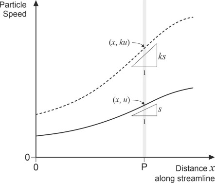
Here we picture a typical fluid element near a moving body. We want to know how the inertial component of the fluid forces acting on it varies with the speed and size of the body concerned. To do this, we’ll carry out a thought experiment in which the fluid has constant density \(\rho\) and the body travels at constant velocity \(V\) relative to the fluid mass (actually, we’ll picture the vehicle as stationary and the fluid as a whole moving at velocity \(V\), but this doesn’t affect the results). We’ll focus on a fluid particle of mass \(m\) located at a point P near the vehicle, and work out an expression for the overall force acting on the particle in its direction of motion along the streamline. As the fluid moves around the vehicle body, the velocity \(u\) of the particle will change continuously as shown by the solid curve in figure 6, as will the rate of change \(du / dx\) of the velocity with respect to distance \(x\) measured along the streamline. Denote by \(s\) the numerical value of this rate of change, equal to the slope of the solid curve in figure 6. Unless \(s\) is equal to zero, the particle will be accelerating or decelerating. This can only happen as a consequence of the various forces applied to it, whose combined effect we’ll denote by \(F_{inertia}\). According to Newton’s second law, the magnitude of this force must equal the particle’s mass \(m\) times its acceleration \(a\) in the direction of the applied force:
(19)
\[\begin{equation} F_{\text{inertia}} \quad = \quad m a \end{equation}\]Here we’ll need to express the acceleration in terms of the well-known formula
(20)
\[\begin{equation} a \quad = \quad u\frac{du}{dx} \end{equation}\]so we can write the result as
(21)
\[\begin{equation} F_{\text{inertia}} \quad = \quad m u \frac{du}{dx} \end{equation}\]Now suppose that the experiment is repeated, this time with a different vehicle velocity \(V' = k V\), given that all other parameters including the size and shape of the vehicle body remain unchanged. The fluid velocity at every point in the flow field will change by the same factor \(k\), whose value for the sake of argument we’ll assume to be greater than 1 though this isn’t essential to the argument. The inertia force acting on the particle will change to a new value \(F'_{inertia}\). If we examine the particle’s trajectory we’ll find that its velocity has shifted upwards to the dashed line in figure 6. At the moment when it passes through the point P its velocity \(u'\) will be equal to \(ku\), and the slope \(du'/ dx\) of the curve will be equal to \(k du / dx\). The acceleration \(du'/ dx\) must therefore be equal to \(\left( k u \right) \times \left( kdu / dx \right) = k^{2} u . du/dx\) so that the new inertia force is given by
(22)
\[\begin{equation} F'_{\text{inertia}} \quad = \quad k^{2} m u \frac{du}{dx} \end{equation}\]In other words, the inertia force on the particle in the direction of motion has increased by a factor \(k^2\) and must therefore be proportional to \(V^2\).
Figure 7
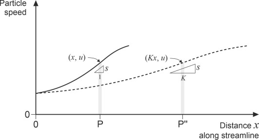
So what about the effect of vehicle size? It’s convenient to measure the size of a moving body in terms of its overall length \(l\), although for our purposes any other dimension would do. Let’s repeat the thought experiment this time with the velocity \(V\) held constant but all the dimensions of the body together with the geometric patterns of fluid motion scaled up by a factor \(K\) so that the body’s length is now \(K l\). Because the body and its surrounding flow field have expanded in 3-dimensional space, the volume of the fluid element under consideration increases in the same proportion so its mass now becomes \(K^{3} m\). Now let’s examine its velocity profile, denoting the velocity at distance \(x\) by \(u''\). The profile is stretched out along the \(x\)-axis as shown in figure 7, with the reference point P moving to a new location P\(''\) whose distance from the origin measured along the streamline becomes \(Kx\). Here, the particle velocity is unchanged, but the slope \(du'' / dx\) of the curve will be equal to \(\left( du / dx \right) / K\). The acceleration \(u'' du''/ dx\) will be \(\left( u \right) \times \left( du / dx \right)/K = u . \left( du /dx \right) / K\) so that the new inertia force is given by
(23)
\[\begin{equation} {F''}_{\text{inertia}} \quad = \quad \left( K^{3} m \right).u \left( \frac{du}{dx} \right) / K \quad = \quad K^{2} m u \frac{du}{dx} \end{equation}\]In other words, the inertia force on the particle has increased by a factor \(K^2\), and therefore must be proportional to \(l^2\), the square of the vehicle size.
Finally, consider the effect of changing the density \(\rho\) of the fluid. This will change the mass \(m\) of the fluid element in direct proportion, so we can say straight away that the inertia force varies in direct proportion to \(\rho\) . Putting this together with the earlier results, we conclude that the inertia force on the fluid element obeys the following ‘scaling rule’:
(24)
\[\begin{equation} \text{Inertial force} \quad \propto \quad \rho V^{2} l^{2} \end{equation}\]Appendix 2: Dimensional analysis of ship resistance
The aim of this Appendix is to find an expression for the resistance or drag \(D\) that opposes a ship’s motion in calm water. There are several variants of the basic technique and we’ll use Rayleigh’s method but describe it in a less formal way than most textbooks. Assume that the relevant variables are the drag \(D\) itself, the acceleration \(g\) due to gravity, the density \(\rho\) of salt water, its kinematic viscosity \(\nu\), the velocity \(V\) of the vessel, and its waterline length \(l\). We start by creating a new set of dimensionless variables from the original ones. To be more specific, they are dimensionless products sharing a common basic structure in which each of the original variables is raised to a power thus:
(25)
\[\begin{equation} D^{ \alpha } l^{ \beta } \rho^{ \gamma } \nu^{ \delta } V^{ \varepsilon } g^{\zeta } \end{equation}\]Let’s focus on one of these new variables. Its constituent terms have six exponents \(\alpha\), \(\beta\), \(\gamma\), \(\delta\), \(\varepsilon\), and \(\zeta\) whose values we don’t know, but we can learn something about them if we replace the quantities \(D\), \(l\), \(\rho\), \(\nu\), \(V\) and \(g\) with the categories of unit in which they are measured: mass \(M\), length \(L\), and time \(T\). This operation is signified by the square brackets in the following equation:
\(\left[ D^{\alpha } l^{\beta } \rho^{\gamma } \nu^{\delta } V^{ \varepsilon } g^{\zeta } \right] \quad = \quad \left( MLT^{-2} \right)^{\alpha } L^{ \beta } {\left( ML^{-3} \right)}^{\gamma } {\left( L^{2} T^{-1} \right)}^{ \delta } {\left( LT^{-1} \right)}^{\varepsilon } {\left( LT^{-2} \right)}^{\zeta }\)After collecting like terms, this becomes
(26)
\[\begin{equation} \left[ D^{\alpha } l^{\beta } \rho^{\gamma } \nu^{\delta } V^{ \varepsilon } g^{\zeta } \right] \quad = M^{ \alpha + \gamma } L^{ \alpha + \beta -3\gamma + 2\delta + \varepsilon + \zeta } T^{-2\alpha - \delta - \varepsilon - 2\zeta } \end{equation}\]By definition the product is dimensionless so we can equate the power of \(M\) to zero, then similarly equate the power of \(L\) to zero, and finally the power of \(T\) likewise, to get the following equations for the indices:
(27)
\[\begin{equation} \alpha + \gamma \quad = \quad 0 \end{equation}\](28)
\[\begin{equation} \alpha + \beta - 3\gamma + 2\delta + \varepsilon + \zeta \quad = \quad 0 \end{equation}\](29)
\[\begin{equation} -2\alpha - \delta - \varepsilon - 2\zeta \quad = \quad 0 \end{equation}\]Here we see three equations for 6 unknowns, which can be solved for any combination of 3 unknowns in terms of the other three. There are fifteen possible ways of doing this (6 times 5 divided by 2). They all lead to the same answer and we’ll solve in terms of \(\alpha\), \(\delta\), and \(\zeta\) because this particular combination makes the arithmetic easy. We have from equations equation 27 and equation 29:
(30)
\[\begin{equation} \gamma \quad = \quad -\alpha \end{equation}\](31)
\[\begin{equation} \varepsilon \quad = \quad - 2\alpha - \delta - 2\zeta \end{equation}\]and after a little manipulation:
(32)
\[\begin{equation} \beta \quad = \quad - 2\alpha - \delta + \zeta \end{equation}\]Substituting these expressions for \(\beta\), \(\gamma\), and \(\varepsilon\) in our structural template (equation 25) yields:
(33)
\[\begin{equation} D^{\alpha } l^{ -2\alpha - \delta + \zeta } { \rho }^{ -\alpha } { \nu }^{\delta } V^{ -2\alpha - \delta - 2\zeta } g^{\zeta } \end{equation}\]If we collect like terms, this becomes:
(34)
\[\begin{equation} {\left( \frac{D}{ \rho V^{2} l^2} \right)}^{ \alpha } {\left( \frac{\nu }{Vl} \right)}^{ \delta } {\left( \frac{gl}{V^2} \right)}^{\zeta } \end{equation}\]This is the template for all of the dimensionless products we are seeking; we can vary the indices \(\alpha\), \(\delta\), and \(\zeta\) to generate each of them in turn. There are infinitely many combinations of \(\alpha\), \(\delta\), and \(\zeta\) to choose from, so in principle we could produce an infinitely large number of candidates. But the aim of dimensional analysis is to condense the original set of variables into the smallest possible set. Our dimensionless products must therefore be mathematically independent (meaning that that none can be created by combining other members of the set), while capable of reproducing all possible products of the original variables. These conditions will be met if we proceed as follows. Start by putting \(\alpha = 1\), \(\delta = 0\), and \(\zeta = 0\), which leaves us with \(D/ \left( \rho V^{2} l^{2} \right)\), our first new dimensionless variable (\(\alpha\) doesn’t have to be 1, it can be any real non-zero number we like). Next, we’ll put \(\delta = 1\) with \(\alpha\) and \(\zeta\) both zero, which generates the second dimensionless variable \(\nu / V l\). Finally, we get the third dimensionless variable \(gl / V^2\) by putting \(\zeta = 1\) and the other exponents equal to zero.
To summarise, we have encapsulated all possible relationships among the seven initial variables in terms of just three non-dimensional variables
(35)
\[\begin{equation} \left( \frac{D}{ \rho V^{2} l^{2} } \right),\quad \left( \frac{\nu }{Vl} \right), \quad \text{and} \left( \frac{gl}{V^2} \right) \end{equation}\]The first is a dimensionless form of the variable in which we are interested, our ‘target’ if you like. The second quantity \(\nu / Vl\) is the inverse of the Reynolds number Re, while \(gl / V^2\) is the inverse of the square of the Froude number Fr. Accordingly, we can express our target variable as a function \(\phi \left( . \right)\) of Re and Fr thus:
(36)
\[\begin{equation} \frac{D}{ \rho V^{2} l^{2}} \quad = \quad \phi \left( \text{Re,} \text{Fr} \right) \end{equation}\]As it stands, both sides of the equation are dimensionless, but if we want, we can write it in a more familiar guise as the classical drag formula
(37)
\[\begin{equation} D \quad = \quad \frac{1}{2} \rho V^{2} l^{2} f\left( \text{Re,} \text{Fr} \right) \end{equation}\]Acknowledgements
Figure 5: Image of CFD mesh created by Envenio software (http://envenio.com), by kind permission of the Design Engineering digital magazine (https://www.design-engineering.com).