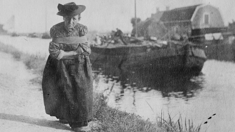
© Bain News Service ca 1910
M.1619
Resistance
A thousand years ago, travelling over land was tedious and slow. By comparison, boats were quicker. In good weather a sailing craft could maintain a steady speed for hours or even days at a time. But during the nineteenth century, new forms of transport began to emerge: roads and railways enabled vehicles to move under their own power, and the first flying machines arrived shortly after. Although slow and unreliable at first, their performance improved rapidly so that within a few decades, travel speeds by land and air had increased roughly tenfold. In the meantime, ships achieved only a modest improvement, so that today, cargo vessels and cruise liners are moving little faster than they did generations ago. There are two reasons for this. First, ships are big. Fully loaded, a crude oil carrier weighs over half-a-million tonnes, the equivalent of around a thousand jumbo jets. Second, when a ship moves, it must push aside a lot of water, which is a relatively dense fluid. At low speeds, the resistance is small, but it rises rapidly above 20 knots and greatly adds to the cost of operation. In this Section, we’ll ask where the resistance comes from, and what can be done to reduce it.
Where resistance comes from
At low speeds, a ship’s resistance is small, comparable with that of a railway train, so that a cargo vessel will cruise economically when travelling at the sort of speed you and I can manage on a bicycle. But if you want it to go faster, the water will exert a significant ‘drag’ that effectively limits the cruising speed to a value that depends on the size of the hull. The level of drag also depends on the depth of water in which the ship is moving: in shallow water or in a narrow channel the fluid accelerates as it squeezes underneath the hull or around the sides, and the resistance increases accordingly. In addition, the resistance increases in rough water, because rolling and pitching motions continually disturb the pattern of flow around the ship’s hull. Let’s start by assuming deep water under calm weather conditions, break down the resistance into its various components, and examine them one by one.
Wave-making resistance
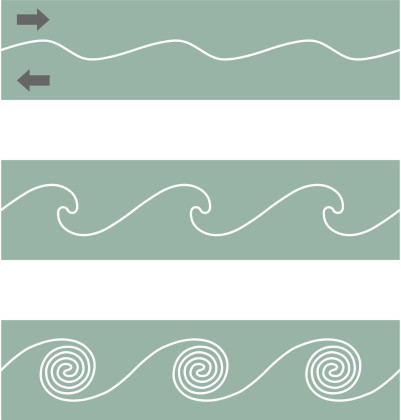
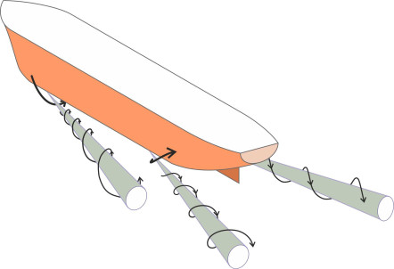
The first component is wave-making resistance. We came across it in Section M1620. It is unique to floating vehicles, and it occurs because a ship moves along the interface between two fluids. If the ship were totally submerged like a submarine, the pressure disturbances would still occur but they wouldn’t generate surface waves and there would be no wave drag at all. Unlike the ordinary waves that travel across the sea under the action of the wind, a ship’s waves are attached to the hull and move along at the same speed. As shown in Section M1620, they fall into a regular geometrical pattern (figure 1), and in plan view, the pattern is pretty much the same for vessels of all shapes and sizes provided they are travelling at a modest speed.
Figure 1
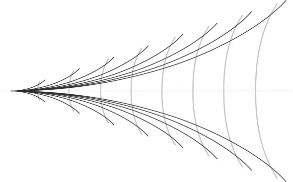
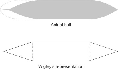
The fluid particles in a surface wave are not actually carried along with the crest, but orbit around fixed positions as described in Section M1620, so when we say that a wave ‘moves’ at a certain speed, the movement we are describing is an illusion. And yet the waves radiate energy away from the vessel that can’t be recovered, and it is the loss of energy that accounts for wave-making resistance. As you might imagine, this resistance varies with the speed of the ship. At low speeds it is almost negligible, but it grows rapidly with speed until it dominates all other resistance components. Shipbuilders would dearly like to have a formula from which they can predict its value for any new vessel before it leaves the drawing board. Well over 100 years ago, scientists tried to solve the problem theoretically. A real ship’s hull was too complicated so they concentrated on idealised geometrical shapes. The first breakthrough came in 1898 when the Australian mathematician J M Michell worked out a formula for a long, narrow hull. Essentially a stick with parallel sides, it was represented as a point source at the bow and a sink at the stern: in other words, the bow radiated waves from a single point, while the stern behaved in the same way except that the waves were of opposite phase [3] [13] [23]. The analysis was later extended by Wigley, who represented the hull in a more realistic way, as a wedge-shaped bow, a wedge-shaped stern, and a parallel middle section (figure 2). In essence he replaced the point source at the bow by two continuous lines of disturbance angled outwards along either side, and treated the stern similarly. In this way he was able to estimate resistance as a function of the Froude number for high-speed monohulls. You can find some results in [13], which display humps and hollows corresponding roughly to those mentioned earlier in Section M1620. But unfortunately, for real ships the wave-making resistance is sensitive to small variations in the shape of the hull: there is no formula that works in every case, and designers usually resort to model tank tests or computer simulation instead.
Figure 2
Frictional resistance
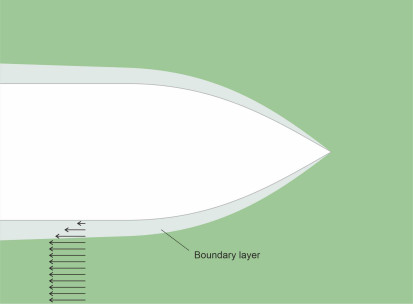
The second component of resistance arises from fluid friction. The way in which a ship’s hull generates friction when it moves through the water is complex and fascinating. It’s not like a cup sliding across your kitchen table, for example, where the two surfaces rub against one another. The process involves a whole layer of fluid close to the hull surface as shown in figure 3. The affected fluid is called the boundary layer. We have already come across the phenomenon in Section C1416 in connection with the flow of air around the body of an automobile, and you’ll find a more detailed decription in Section F1917. In fact, any rigid body moving through a fluid will affect nearby fluid particles through molecular attraction, so that on a microscopic scale, they adhere to the body surface, even if the surface is perfectly smooth. Since all fluids are viscous to a greater or lesser degree, these particles will in turn influence those further away, so that neighbouring layers of fluid are dragged along with the moving body at a velocity that diminishes with distance. The rate at which the velocity falls with increasing distance is called the velocity gradient.
Figure 3
So far, we haven’t said much about the way individual particles might be moving. A non-zero velocity gradient implies that any ‘packet’ of fluid sliding along a rigid body surface undergoes a shearing action, so that the particles close to the body surface are travelling at a different speed from those further away. But are they travelling along a smooth curve parallel to the surface, in other words, along well-defined streamlines? Such a condition is known as laminar flow, and experiments have shown that such motion is possible over a limited distance provided the fluid is sufficiently viscous to damp down random perturbations, and provided the velocity gradient is not too severe.
For moving vehicles this is not usually the case. As the layers shear over one another the interface between them changes from a smooth, flat plane to a wavy, rippled one, a process that echoes the way that the wind creates waves on an otherwise calm pond (figure 4). The waves curl over and roll into eddies, so that neighbouring layers intermix and exchange energy, and the flow is said to become turbulent. Exactly what shape the eddies take and how they interact with one another is not clearly understood. It’s hard to track what goes on inside a fluid at a microscopic level, and after more than 100 years of effort, the mathematical representation of turbulent flow still remains a challenging field. What we do know is that during the transition, the boundary layer on the surface of a moving vessel thickens and the frictional resistance increases, so it’s important for the marine architect to know which type of motion, laminar or turbulent, is likely to occur.
Figure 4
There’s a neat way to find out. It involves the Reynolds number \(Vl/\nu\), in which \(V\) is the velocity of the vessel, and \(\nu\) the kinematic viscosity. During the nineteenth century, Reynolds discovered that a fluid in a pipe switched from laminar to turbulent flow when this number reached a threshold of around 2000, and you can find out more about his work in Section F1917. For a moving vehicle immersed in a fluid, we interpret \(l\) as the distance measured longitudinally along the body surface from the nose, and \(V\) as the velocity of the undisturbed stream. Experience has shown that here, the critical value of Reynolds number at which the flow becomes turbulent is around \(5 \times 10^{5}\) [22]. So what conditions do we find in the boundary layer of a moving ship? Imagine a 400 m-long crude oil carrier Alba cruising at 12 knots (6.177 m/s) in seawater whose kinematic viscosity is \(1.188 \times 10^{-6} \text{ m}^{2} \text{/s}\). Starting at the bow where \(l\) is zero and Re is zero, the flow is laminar but the laminar flow doesn’t persist for long. The distance \(l_\text{crit}\) at which it becomes turbulent is given by \(\nu \times \text{Re} / V\), which in this case is \(\left( 1.188 \times 10^{-6} \right) \times \left( 5 \times 10^{5} \right) / 6.177 = 0.096 \text{ m}\). In other words, the transition occurs only 10 centimetres from the bow, and the boundary layer is turbulent for almost the whole length of the hull. At the stern, the Reynolds number reaches a value equal to \(400 \times 6.177 \times 10^{6} / 1.188 = 2.079 \times 10^{9}\), and indeed we find that for large vessels, values of the order of \(10^{9}\) are common [1]. Incidentally, the boundary layer grows thicker as the particles travel along the hull surface, and for a container vessel it may reach a thickness of 1m at the stern.
Figure 5
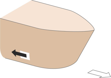
Figure 6
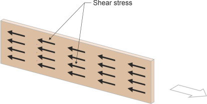
Just as the hull exerts a force on the boundary layer (dragging it along in the direction of motion), so the boundary layer exerts an equal and opposite force on the hull. Over each square centimetre of the hull surface, it’s a shear force acting parallel to the skin (figure 5). The sum of these shear forces, or more correctly their components resolved parallel to the longitudinal axis of the ship, is equal to the frictional resistance. Its value is roughly proportional to the wetted surface area below the waterline. Hence one can predict the frictional resistance of a ship by likening the hull to a flat plank being towed along under the surface (figure 6). Like most hydrodynamic forces, the frictional resistance \(R_F\) of a flat plate obeys a relatively simple equation [25]:
(1)
\[\begin{equation} R_F \quad = \quad \frac{1}{2} \rho V^{2} S C_F \end{equation}\]where \(\rho\) is the mass density of seawater, \(V\) is the velocity of the plate, \(S\) is the total wetted area, and \(C_F\) is the friction coefficient. It would be convenient if \(C_F\) were constant, but in reality, it’s not: the drag increases with the Reynolds number. Hence the problem hinges on the relationship between \(C_F\) and Re.
In the past, shipyards and design offices worldwide assumed different relationships, which sometimes led to inconsistent estimates for the same hull configuration. Eventually, an association called the International Towing Tank Conference (ITTC) was formed to standardise procedure. In 1957 the ITTC adopted the following formula for a smooth hull surface that effectively compensated for the variation in Re [25]:
(2)
\[\begin{equation} C_{F} \quad = \quad \frac{0.075}{ \left[ \log_{10} \left( \text{Re} \right) - 2 \right]^{2} } \end{equation}\]Using this formula together with equation 1 we can get a rough estimate of the frictional resistance for any ship hull if we know the wetted area, i.e., the surface area of the hull below the waterline. Let’s return to our crude oil carrier Alba, and suppose that with a beam of 40 m and loaded draft of 15.5 m she has a wetted surface area of \(25 000 \text{ m}^2\). We calculated earlier that when cruising at 12 knots the Reynolds number at the stern came to \(2.079 \times 10^9\). Hence from equation 2 we can work out the friction drag coefficient, which comes to around 0.00140. Assuming a seawater density of \(1025 \text{ kg/m}^3\), when substituted back in equation 1 we get a friction resistance value of \(0.5 \times 1025 \times 25 000 \times 6.1772 \times 0.00140\), roughly 685 kilonewtons. This is equivalent to a weight of just under 70 tonnes.
The basic formula assumes that the hull surface is smooth, whereas in practice it’s not. If you examine almost any ship below the waterline you’ll find small deformations in the plating together with flaking paint and corrosion, and worse, and after a little time at sea, the hull becomes coated with organic matter: bacteria and diatoms followed by algae and barnacles or mussels [6]. Surface roughness of this kind causes extra drag and can increase fuel consumption by \(40\%\). Fouling occurs very quickly, and in one experiment, it was found to increase a ship’s frictional resistance at a rate of almost \(1\%\) per week [27]. We won’t go into detail here, but a modified version of the formula for \(C_F\) allows for fouling, and also for the fact that water flows round the sides of a three-dimensional hull more quickly than it does along a flat plank of the same area, so the resistance is higher than equation 2 would suggest.
Pressure drag or form drag
The third main component is the pressure drag, otherwise known as the form drag. It is created by the pressure of the water acting on each part of the hull at right-angles to its surface (figure 7), and is equal to the sum of the components resolved in the direction of the longitudinal axis of the hull. As explained in Section F1817, all vehicles are subject to pressure drag, but in the case of a ship it rarely accounts for more than a small proportion of the total resistance, being dominated by the wave-making resistance at speeds above 4-5 knots. Most of it arises because the water flow separates from the hull surface where the sides curve inwards towards the stern, creating a confused wake or ‘deadwater’ region where the pressure is reduced [26]. In addition, the hull can generate a vortex on either side of the bow [15] where the boundary layer descends around the bilges and breaks away. The reverse happens at the stern where the boundary layer ascends round the bilges as it converges towards the propeller or propellers. Figure 8 shows the bow and stern vortices on the port side of the hull. These vortices seem to mirror the ones generated by the A-pillars and the C-pillars of a saloon car body as described in Sections C1416 and F1818.
Figure 7
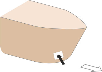
Figure 8
Other forms of resistance
The remaining components are smaller still. Appendage resistance arises from fittings such as the propeller shaft and rudder that project beyond the smooth envelope of the hull. Typically it accounts for \(10\%\) of the total [3] [26]. Its value is difficult to predict, nor is it easy to measure in a towing tank. One must first test a model of the hull stripped bare of all appendages, then add the appendages and test it again. When scaled down to model size, an appendage may be so thin and delicate that it buckles or deforms under the pressure of the fluid flow [24]. Also the Reynolds number for each appendage varies according to its size, and its resistance doesn’t scale up correctly to the full sized ship. In practice therefore, a designer will use an empirical formula instead.
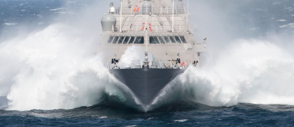
The next component is spray resistance. In addition to making waves, a vessel throws up a greater or lesser quantity of spray, which carries away energy. The energy loss accounts for a small component of the resistance for a slow-moving vessel such as a cargo ship, but it’s more significant for faster vessels [11]. You’ll have seen how a powerful speedboat generates a bow wave under the V-shaped bottom of its planing hull, which is designed to expel the fluid outwards rather than curving upwards around the bilges. When impacted by the hull, the water has nowhere else to go. At its root is a ‘solid’ sheet of fluid that bursts violently out of the surface as explained earlier in Section M1718. The sheet then disintegrates into ‘white spray’ (a mixture of water droplets and air). Even more spectacular is the bow wave formed by a large, fast-moving semi-displacement hull with a rounded bilge such as a naval destroyer (figure 9). Because the sides are nearly vertical, the bow wave exits almost vertically from the water surface.
Figure 9
Finally, we come to air resistance, which is typically between 2 and \(4\%\) of total resistance, and more for container ships and fast ferries. A headwind increases the air resistance and slows the ship down in the same way that it does for cars, trains and other land vehicles. We won’t go into detail here, but you can find more information in the standard textbooks [28]. Sea waves also have an effect. They bludgeon the vessel and disturb the steady pattern of flow round the hull, creating extra drag.
Disentangling the components
Estimating the resistance for any particular vessel seems a daunting task given the number of separate components involved. A similar problem arises in other fields, so let’s start by asking how an automobile engineer might tackle the problem. The air resistance of an automobile has two key components (friction drag and pressure drag) that can be lumped into a single equation as described in Section C1416:
(3)
\[\begin{equation} \text{Drag or resistance} R \quad = \quad \frac{1}{2} \rho V^{2} A C_D \end{equation}\]where \(\rho\) is the density of air, \(V\) is the wind speed relative to the vehicle, \(A\) is the cross-sectional area of the vehicle body, and \(C_D\) is the drag coefficient. Within the range of conditions under which the formula is usually applied, the value of \(C_D\) is almost constant. It tells you how the shape of the body affects the drag, independently of its size. The effect of size is expressed by the frontal area \(A\). This division of roles is both neat and useful because it allows the designer to make predictions from experiments with relatively small models.
In fact, equation 3 is a simplified version of a more general equation that applies across the whole field of fluid dynamics. You’ll find the equation and further details in Section F1817. But here we are dealing with ships, whose behaviour in some respects is unique. Ships make waves, and as we saw in Section M1620, any interaction between the bow and stern systems distorts the relationship between resistance and speed, introducing ‘humps’ and ‘hollows’ so that \(R\) no longer increases smoothly as \(V^2\). The drag coefficient \(C_D\) is certainly not a constant.
The scaling problem
So given that we want to build a ship of any particular size and shape, how do we determine the drag coefficient? The obvious method is to build a model and test it in a water tank. By measuring the drag at an appropriate model speed we can use equation 3 to work out the drag coefficient and then apply it to the full-size ship. However for the results to have any meaning two conditions must be satisfied: the model and ship must operate (a) at the same Froude number and (b) at the same Reynolds number. Only when these two conditions are satisfied will the wave-making resistance and the frictional resistance component both scale up correctly to their full size values.
Unfortunately, one can’t achieve both at the same time. We can see this with the aid of an example. Consider a ship whose hull length \(l_s\) is 100 m and whose cruising speed \(V_s\) is 12 knots (equivalent to 6.18 m/s). We want to estimate its wave-making resistance by testing a scale model whose hull length \(l_m\) equals 5.0 m. Let \(V_m\) be the speed at which the model travels through the towing tank. The Froude number for the ship is given by
(4)
\[\begin{equation} \frac{V_s}{\sqrt{g l_s}} \quad = \quad \frac{6.18}{\sqrt{9.81 \times 100}} \quad = \quad 0.197 \text{ approx.} \end{equation}\]To work out the Reynolds number we shall need a representative value for the kinematic viscosity of water, which varies with salinity and temperature. Let’s assume that the ship operates in salt water at a temperature of \(15^{\circ} \text{C}\): the kinematic viscosity will then be \(1.188 \times 10^{-6} \text{ m}^{2}/\text{s}\) and the Reynolds number
(5)
\[\begin{equation} \frac{V_{s} l_{s}}{\nu} \quad = \quad \frac{6.18 \times 100}{1.188 \times 10^{-6}} \quad = \quad 0.520 \times 10^{9} \text{ approx.} \end{equation}\]Since the towing tank must operate at the same Froude number as the full-sized ship we know that the speed of the model \(V_m\) through the water must satisfy
(6)
\[\begin{equation} \frac{V_m}{\sqrt{g l_m}} \quad = \quad \frac{V_m}{\sqrt{9.81 \times 5}} \quad = \quad 0.197 \end{equation}\]so that \(V_m\) is \(0.197 \times (9.81 \times 5)^{0.5}\) or 1.38 m/s. The towing tank will be fresh water at say \(20^{\circ}\)C for which the kinematic viscosity is \(1.004 \times 10^{-6} \text{ m}^{2}\)/s. Hence the Reynolds number for the model will be
(7)
\[\begin{equation} \frac{V_{m} l_{m}}{\nu} \quad = \quad \frac{1.38 \times 5}{1.004 \times 10^{-6}} \quad = \quad 6.87 \times 10^{6} \text{ approx.} \end{equation}\]which is too small by a factor of nearly a hundred. It follows that a towing tank test will reproduce the wave-making resistance correctly but the frictional resistance component will be wide of the mark. Of course we could abandon the Froude number requirement and equalise the Reynolds number instead, which would imply a model speed satisfying
(8)
\[\begin{equation} \frac{V_{m} l_{m}}{\nu} \quad = \quad \frac{V_{m} \times 5}{1.004 \times 10^{-6}} \quad = \quad 0.520 \times 10^{9} \text{ approx.} \end{equation}\]in which case \(V_m\) comes to \(\left( 0.520 \times 10^{9} \right) \times \left( 1.004 \times 10^{-6} \right)/5 = 104\) m/s, over 200 knots. Even if we could get the water in the tank to flow that fast, the Froude number would be wrong by a large factor and the wave-making resistance wide of the mark. To summarise, the friction and wave-making components do not scale up in the same ratio, which makes it impossible to judge the full-size ship from a model test. During the Victorian era this made ship design a rather uncertain business. Lacking a sound basis for estimating the resistance, the marine architect could not with any certainty judge the engine power needed to achieve the required cruising speed. It seemed the only way to get reliable results was to build the ship first and measure its resistance by towing it through the water and measuring the pull on the cable. However, a mathematically gifted engineer called William Froude found a better way.
Figure 10
Froude’s method
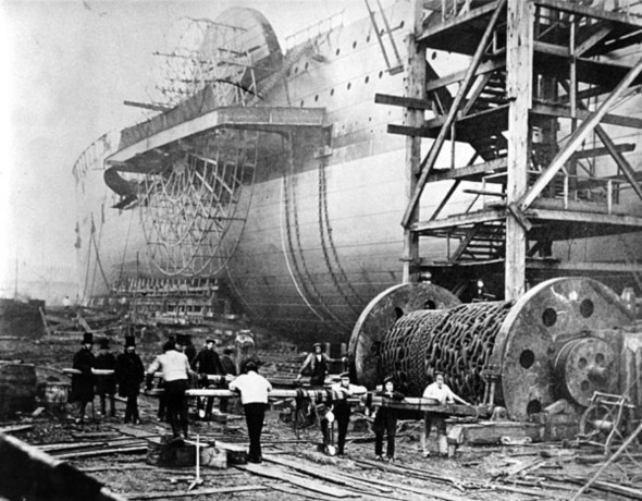
William Froude (1810-1879) was a close friend of Isambard Kingdom Brunel, and had worked with him on the S S Great Eastern. Built at Millwall on the River Thames in London, the Great Eastern was by far the largest ship afloat at the time of her launch in 1858 (figure 10). Although it was a commercial failure, the experience stimulated Froude’s interest in the behaviour of ships under power. He was the first to realise that a model of geometrically similar form to a real ship would create a similar wave system, but to do so it would have to travel at a different speed. Supposing as before that the ship is moving at speed \(V_s\). The speed \(V_m\) of the model, which he called the ‘corresponding speed’, must then be scaled in proportion to the square root of the ratio of the waterline lengths:
(9)
\[\begin{equation} \frac{V_m}{V_s} \quad = \quad \sqrt{\frac{l_m}{l_s}} \end{equation}\]For the rationale behind this assertion, you might wish to refer to Section M1620. In theory it enabled the designer to estimate the resistance of a ship by measuring the resistance of a model and scaling up the result. Froude was convinced that he could do this if the total resistance were split into two main components that he called ‘friction’ and ‘residuary’. The friction component didn’t depend so much on the shape of the hull as its size, in particular the surface area. Having a long, slender shape typical of that era, the hull could be treated as a flat plank. Through a series of experiments in the towing tank he arrived at a formula for the frictional resistance \(R_F\) of the plank:
(10)
\[\begin{equation} R_{F} \quad = \quad fSV^n \end{equation}\]where \(f\) was a coefficient that varied with the roughness and length of the plank, \(S\) was the wetted surface area, and \(n\) a dimensionless exponent. The formula could be used to predict the frictional resistance component of a model or a full-size ship purely on the basis of the area of hull in contact with the water. At first sight the formula does not seem consistent with the standard model for fluid resistance as set out in equation 3. The right-hand side of equation 10 is equivalent to a constant times \(S V^n\), and Froude discovered that for frictional resistance, the value \(n = 1.825\) best fitted the ships typical of that time [4]. Compare this with the right-hand side of equation 3, which is equivalent to a constant times \(S V^{2}\). Indeed, it turns out that for ships, the relationship between frictional resistance and velocity is more complex than equation 3 would indicate.
Nevertheless, the procedure worked: it enabled Froude to put aside the frictional component of resistance and to concentrate on the residuary component. His method was to build a scale model and measure the total resistance \(R_m\) when it was towed through a tank of water at the ‘corresponding speed’ (i.e., the speed scaled to produce a wave system similar to that of the vessel under investigation). Then he subtracted the frictional component as estimated from equation 10. This effectively isolated the residuary component \(R_{mR}\) which could be scaled up separately to give an estimate \(R_{sR}\) for the full-sized ship. Finally, he added the frictional resistance for the full-sized ship, again estimated from equation 10, to get the total.
But how to scale up the residuary resistance from a model to a full-sized ship? Two basic facts are needed. First, equation 3 tells us that the residuary resistance is proportional to the square of the speed times the cross-sectional area, which itself is proportional to the length squared. Second, the condition for corresponding speeds as set out in equation 9 requires that the ratio \({V_{s}}^{2} / {V_{m}}^{2}\) must be equal to the ratio of ship length to model length. Put these two facts together and it’s not difficult to work out that the ratio of the two residuary resistances must equal the ratio of the cube of the ship length to the cube of the model length, and these two cubes in turn are proportional to the respective hull volumes thus:
(11)
\[\begin{equation} \frac{R_{sR}}{R_{mR}} \quad = \quad \frac{{l_s}^3}{{l_m}^3} \quad = \quad \frac{\nabla_s}{\nabla_m} \end{equation}\]In other words, you scale up the residuary resistance according to the displacement.
Towing tank tests
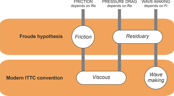
Froude’s procedure enabled marine architects to estimate a ship’s resistance in a scientifically rigorous way. But there were pitfalls, of which we’ll mention only two. First, the residuary component of resistance is a composite of the wave-making and pressure drag. They are uncomfortable bedfellows because wave resistance scales up and down in proportion to displacement whereas pressure drag does not – it varies with Re and does not scale up correctly from model to ship when treated in this way. Like the friction component, pressure drag derives from the viscous nature of water, and ideally it is these two that should be lumped together. Fortunately, in Froude’s day the range of variation was small so any resulting errors were thought to lie within acceptable limits. Second, the assumptions underlying the ‘flat plate’ method of estimating frictional resistance weren’t strictly accurate. The way that water moves around a ship is different from the way it moves across a flat plate. When it curves around the hull, the boundary layer is liable to break away, leaving pockets of confused flow next to the skin, and perhaps vortices as shown earlier in figure 8. Consequently, a better formula was needed that somehow took into account the hull shape.
Today, these issues are resolved by grouping the elements in a different way (figure 11): the total resistance is split into ‘viscous’ and ‘wave-making’ resistance components [2] [20]. The pressure drag is now lumped with the frictional resistance rather than the wave-making resistance, and the sum of the two - the viscous component – is estimated from flat plate friction drag, modified to allow for the curved shape of the hull using a ‘form factor’ [25].
Figure 11
Towing tank tests are still needed to estimate the wave-making resistance of any new vessel. They are carried out at one of a number of specialised centres under guidelines agreed by the International Towing Tank Conference (ITTC) [35]. The towing tank may be over 100 m long and over 5 m wide. The model itself is usually made from wood, GRP or wax, and accurately shaped with a smooth painted finish [24]. Usually between 4 and 10 m long [1], the model is suspended from a cradle that traverses the length of the tank at a speed of anything up to 6 m/s. The cradle is fitted with sensors that measure the hydrodynamic forces acting on the model as it moves along the water surface.
Other methods
Although reliable, model tests are expensive and time-consuming. During the early stages of the design process, before fixing the shape of the hull the designer may want to explore a range of possibilities without going to the expense of building and testing a model for each variation. What is needed is a formula that gives an approximate estimate based on a few geometrical parameters. Acknowledged as the industry standard and widely used in design offices is the procedure developed at the Netherlands’ marine research institute MARIN by J Holtrop and G G J Mennen [17]). It’s not actually a single formula, but suite of regression equations fitted to model data and ship data over a period of many years. Each equation predicts an individual element of resistance as a function of certain explanatory variables that describe (among other things) the hull geometry. We’ll carry out a sample calculation using not the original suite, but a simplified version that reduces the process to a single formula [34] that applies to bulk carriers sailing in calm water (a bulk carrier is a cargo vessel that carries raw material such as oil or mineral ore for example). The formula is
(12)
\[\begin{multline} \frac{R}{V^2} \quad = \quad 3.75 - 0.00000015 L^{3} + 0.00024 B^{2} \ln{B}\\ - 0.00064 T^{3} - 14 {\left[ \ln{C_B} \right]}^{2} + 0.0000173 \nabla \ln{\nabla} \end{multline}\]where \(R\) is the resistance in kN, \(V\) the ship speed in m/s, \(L\) the waterline length in metres, \(B\) the beam in metres, \(T\) the draft in metres, \(C_B\) the block coefficient, and \(\nabla\) the volume displacement in m3. The formula takes no account of air resistance, nor does it reflect the ‘humps and hollows’ in the wave-making resistance profile that arise from interference between the bow and stern wave systems. Bearing this in mind let’s work out a prediction for one of the largest types of bulk carrier. Known as the M4, it has a waterline length of 243 m, the beam is 32.2 m, the draft 11.6 m, the block coefficient 0.815, and the volume displacement 73 900 m3. Substituting these values in equation 12 yields a value of about 15.2 for \(R/V^{2}\), from which we deduce that the resistance is a little under 800 kN at a cruising speed of 7.2 m/s or 14 knots. This is a relatively small force, equivalent to roughly one tenth of a percent of the overall weight of the ship plus cargo.
Regression formulae of this kind are based on the behaviour of existing vessels, and don’t work so well in the case of a radical design for which no data yet exists. Software developers have for some time been working on packages that can simulate fluid flow around a ship’s hull. As you can imagine, it’s not an easy task to represent the interactions among large numbers of fluid particles in turbulent motion. During the 1990s, so-called boundary element methods came close to solving the problem and in principle they could predict hull resistance, but they fell short in certain respects (they did not account properly for breaking waves, for example [1]). More recently, specialised techniques under the general heading of Computational Fluid Dynamics (CFD) have enabled designers to model aircraft and ship behaviour with greater accuracy.
Slippery ships
Over its lifetime, a cargo vessel burns a lot of diesel fuel. You might be surprised to learn that the fuel costs more than the vessel itself. As the largest single item in the operator’s budget, it accounts for \(40\%\) of the total including crew, insurance, and cargo handling charges [30]. So a great deal hangs on the ship’s resistance, and the question is how to reduce it. The problem is not as simple as it looks, because the resistance has several components, each of which varies in a different way with the hull size and shape, so that a hull that performs well in terms of frictional resistance, for example, doesn’t generally have a low wave-making resistance too. So we’ll consider separately the influence of the hull size, then its shape, and conclude with a brief examination of the hull surface.
Hull size
The resistance forces acting on a small boat are different from the ones acting on a large boat, not because they are different in kind, but because a small object has greater surface area in relation to its volume. One can put this in more precise terms: for a hull of a given shape and length \(l\), the wetted surface area is proportional to \(l^2\) while the displacement is proportional to \(l^3\). So if we double its length, the displacement \(\nabla\) will grow by a factor of 8 while the wetted area \(S\) grows by a factor 4, only half as much. Equation 1 tells us that the frictional resistance is proportional to \(S\), hence as the displacement increases, the friction drag increases at a lesser rate. What about the other resistance components? The author’s analysis in Section F1317 suggests that in relation to its displacement, the wave-making drag for a conventional displacement motor vessel increases less quickly still. All round, large ships have less resistance per unit hull capacity than small ones, so if we want to minimise the resistance per tonne of cargo carried, other things being equal, a few large ships will perform better than a multiplicity of smaller ones.
Hull shape
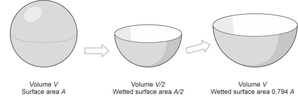
Now let’s fix the hull size and concentrate on its shape. Suppose we wanted to minimise the surface area of the hull: what shape would we choose? An obvious candidate is the sphere, whose surface area \(S\) in relation to its volume displacement \(\nabla\) when submerged is less than that of any other geometrical form. However, a hull shaped like a football that lies submerged below the water surface is neither practical nor optimal. We want some of the vessel to project above the water surface while minimising the area of hull below the waterline, and a better candidate appears to be a hemispherical bowl. If we start by slicing the sphere horizontally in two, the lower half becomes a bowl of displacement \(\nabla / 2\) whose wetted surface area is \(S / 2\). To make this comparable with the original sphere, we need to scale it up as shown in figure 12 so it has the same volume. We do this by increasing its radius by a factor equal to \(2^{1/3}\). This causes the displacement to double, thereby matching the original sphere. At the same time, the surface area will increase by a factor of \(2^{2/3}\), to a value \(2^{2/3} \times \left( S/2 \right)\) or \(2^{-1/3} S\), which is about \(20\%\) less than the original sphere. You might object that this is the worst possible shape for a hull because the ship (a) would be unstable in roll, (b) would be almost impossible to steer on a fixed course, and (c) wouldn’t slice easily through the water so it would generate unnecessary wave-making resistance. Nevertheless there have been special-purpose vessels built almost of this shape. Although shallower than a hemispherical bowl, the coracle has a circular plan form, and at the time of writing is still being used on rivers in Wales for fishing at night. So what about a more practicable form of cargo vessel? In general terms, if it’s not expected to travel fast one might expect such a vessel to be relatively short and wide, with an elliptical cross-section. The cog, a sailing vessel that transported cargo back and forth across the Mediterranean five hundred years ago, had curved bilges together with a length-to-beam ratio of about 3:1. Cargo vessels today still tend to be short and ‘beamy’, with a length-to-width ratio of around 6:1 [14].
Figure 12
For a faster vessel, the situation changes. Wave-making resistance increases sharply with increasing speed and the relative contribution of the frictional component declines, so we’ll need a shape that makes less disturbance when cutting through the water. Let’s start with the cross-section amidships. The main alternatives are a shallow curve such as a semi-ellipse, a ‘V’ section, or a ‘U’ section with vertical sides. Assuming that the cross-sectional area is fixed, both the shallow curve and the V format are wider at the top than the U section and must therefore push aside a greater volume of fluid at the water surface, which implies more wave-making resistance. The U-section or even a rectangular section looks like the best option.
Now for the contours in plan. It’s important that the waterplanes follow a smooth curve from bow to stern because any sharp change in angle will cause additional waves and increased resistance. Traditionally, shipwrights aim for a sharply pointed bow having ‘fine entry lines’ together with a ‘fine run’ at the stern. The cross-sectional area should be small, which implies a relatively long, narrow hull, and in fact a long hull itself confers a speed advantage. From Section M1620 we know that when the Froude number reaches about 0.54, the bow and stern wave systems reinforce one another, which raises the energy dissipated in the wave-making process to a peak. This resistance peak effectively limits the speed of a displacement vessel to a value known as the ‘theoretical hull speed’, which is around \(0.54 \sqrt{gl}\) where \(l\) is the waterline length. The most effective way to overcome the barrier is raise the hull length, which explains why naval destroyers were built during the Second World War with a length-to-beam ratio as high as 10:1 [31], and why the racing sculls (rowing boats) that you see at a regatta are almost absurdly long and slender at 30:1.
However, lengthening the hull doesn’t necessarily reduce the wave-making resistance across the whole range of operating speeds, because it can alter the degree of interaction between the bow and stern wave systems in an unpredictable way. In fact there is no optimum shape for all speeds, only for specific Froude numbers [29]. Furthermore, in a rough sea, a long, narrow hull may be less stable in roll, and may from time to time bridge between extreme waves, which leads to high bending stresses at the keel and deck level: to cater for them requires heavier plating, so the ship will cost more to build while its carrying capacity falls.
So far, we have only looked at frictional and wave-making drag, which between them account for the greater proportion of the total resistance. It’s time to consider the third component: pressure drag. Of all the possible body shapes for a vehicle, the ‘teardrop’ is thought to produce less pressure drag than any other shape. As explained in Section F1616, it has a blunt, rounded nose together with smoothly curved sides and a pointed tail. Contrary to what you might expect, the blunt nose contributes scarcely any drag: it’s the tail that matters, because a gentle taper towards the rear is less likely to cause separation together with a low-pressure wake. Although widely employed in aircraft design, the teardrop works for marine craft too, which is why a nuclear submarine has a rounded nose and a long tail, and presumably why shipwrights at one time, taking their cue from the shape of fish, believed that a teardrop plan form would make their sailing ships faster. Nowadays, the bow is not usually rounded but follows a narrow ‘V’ profile in order to penetrate oncoming waves and reduce their impact in rough water. However, most large vessels have a bulbous bow below the waterline.
Figure 13
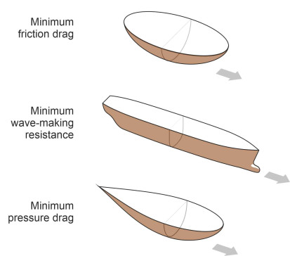
To summarise, a ship’s hull faces a number of conflicting requirements, so that the optimum shape varies according to the size and speed of the vessel concerned. A slow vessel can be short, fat and blunt as shown in figure 13 because this minimises frictional resistance, whereas a fast vessel must be long, thin and pointed at both ends in order to minimise wave-making resistance. And if we look more closely, other factors complicate the picture: for example, a modern cargo ship has a broadly rectangular cross-section because (a) it allows a narrower beam (which further reduces the wave-making resistance), (b) it’s cheaper to build, and (c) it enables the vessel to carry more cargo within a given cross-sectional area of hull. For reasons that are still not properly understood, a bulbous bow reduces resistance for most large vessels independently of the design cruising speed. And container ships are not usually tapered in plan towards the stern: one can achieve a ‘fine run’ in a different way, by sloping the underside of the hull gently upwards towards a transom at the stern. In recent decades, shipbuilders have developed some radical alternatives to the traditional displacement hull, some of which we’ve already touched on (the planing hull, for example) and some of which we’ll introduce later in Section M1506.
The hull surface
For slow-moving vessels, fluid friction accounts for at least half of the total resistance. Earlier we saw how its value increases owing to surface roughness caused by barnacles and other sea organisms. This is why ships need regular cleaning, which during the 1960s, used to take place at frequent intervals. For example the SS France (a famous passenger liner of the day) had its bottom scraped twice a year. Matters have improved somewhat since chemists developed a series of anti-fouling paints [6]. Early ‘organotin’ compounds proved toxic on entering the marine food chain and have since been prohibited by international agreement, but modern coatings are self-polishing and are thought to be safe: they contain a biological agent that is released progressively as the coating wears away, which provides a continuing deterrent to organic fouling.
In tackling the resistance problem, researchers have occasionally been able to learn from the behaviour of aquatic creatures in their natural environment. Some are remarkably efficient. Dolphins are a good example – they will often race alongside a ship, apparently for sheer enjoyment. It’s been suggested that a dolphin experiences less resistance than theory would predict, that is to say, less than a rigid body of the same size and shape. Photographs have revealed ripples on its skin when it approaches maximum speed, presumably damped by the glutinous layer beneath. If so, this might reduce the friction drag. An undulating surface can absorb some of the energy associated with eddies in the boundary layer and by damping down turbulence, sustain laminar flow beyond the speed at which turbulence normally arises. In the late 1950s, this idea was pursued by a German research scientist Dr. Max Kramer, who had previously helped to develop guided projectiles during the Second World War. Later he founded a company in the USA to develop an artificial skin Lamiflo for underwater vehicles with properties similar to those of a live dolphin [19]. It was claimed to reduce drag by up to 30%. Some have disputed this claim, but recent research seems to show that a compliant coating can indeed postpone the transition from laminar to turbulent flow, and therefore that a reduction in drag is possible [7].
Even if the hull surface is rigid, one can manipulate the boundary layer in other ways. The US National Aeronautics and Space Administration NASA discovered that fine grooves running in the direction of the flow reduced friction slightly. When applied to the 1988 America’s Cup winner in the form of adhesive sheets, the grooves reduced drag by 2% [10], probably by interfering with the development of the microscopic ‘hairpin vortices’ on the hull surface that precede turbulence [18].
Conclusion
We’ve seen that fuel accounts for a major share of the cost of shipping, and by implication, that fluid resistance has an appreciable impact on the economics of global trade. Compared with other vehicles, ships are unusual in the sense that when travelling slowly, the resistance they experience is relatively small, less than that of a railway train carrying an equivalent load - because a railway train needs a significant force to overcome the ‘starting resistance’ and get the wagons rolling. On the other hand, a ship’s resistance increases rapidly with speed, and large ships use diesel fuel that is dirty and contributes significantly to global warming, accounting for 3 – 4% of the world’s CO2 production [5]. This won’t be an easy problem to resolve. To achieve a significant reduction in the short term, several measures will be needed in combination, including possibly cleaner fuel, assistance from wind power, a general reduction in operating speeds, and the construction of larger ships that by virtue of their size alone, burn less fuel per tonne-kilometre of cargo carried. The picture for smaller vessels is more encouraging, because they are already evolving in a more radical way. As we’ll see in Section M1506, inventors are producing new hull configurations for fast ferries, patrol boats, leisure craft, and even fishing boats, all aimed at reducing resistance by transforming the relationship between the hull and the water.
Acknowledgments
Photo on opening page: Bain News Service ca 1910, US Library of Congress, posted at https://commons.wikimedia.org/wiki/File:Holland_-_woman_drawing_canal_boat_(pulling)_LCCN2014697180.jpg (accessed 12 May 2021).
Figure 09: USS Milwaukee, from a video produced by Marinette Marine, by kind permission of Fincantieri Marine and Lockheed Martin, 25 September 2016.
Figure 10: Image posted at https://commons.wikimedia.org/wiki/File:Great_eastern_launch_attempt.jpg (public domain, accessed 12 May 2021).