F.1317
Big is beautiful
When you travel, your vehicle will meet resistance from its surroundings, in particular, resistance from the fluid through which it moves. The fluid might be air or it might be water, and in some cases both, but your vehicle must push it aside to reach your destination. The resistance varies from one vehicle to the next because different kinds of vehicle travel at different speeds and have different characteristic shapes: a racing car penetrates the air quite easily because it is long and slender, while a truck is short and squat, and causes more aerodynamic disturbance in relation to its size. As an engineer would put it, the racing car wins because it is ‘streamlined’. Earlier in Section F1616 we explored different body shapes and showed how their influence could be expressed in terms of a single number: the drag coefficient. In this Section, we’ll turn to a closely related question: that of vehicle size.
Figure 1
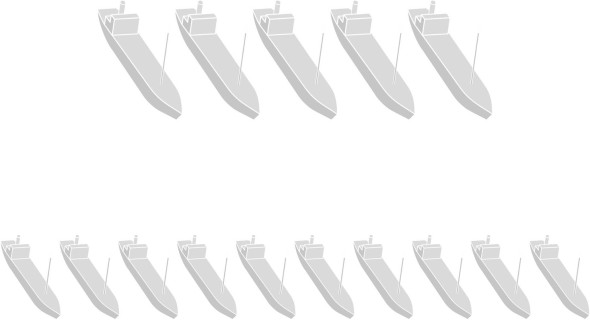
It’s obvious that other things being equal, a large vehicle suffers more drag than a small one, and burns more fuel on any particular trip. But does it burn more fuel in relation to the load it is carrying? It’s an important question because a fleet operator may be able to reduce operating costs and carbon emissions by upsizing. Imagine you are planning to run a cargo service across the Pacific Ocean. In principle, you might employ 10 small vessels, or 5 large ones each of twice the carrying capacity (figure 1). There are many reasons for preferring large vehicles, and no doubt many reasons for preferring small ones, but here we are concerned with one specific issue: which fleet would consume less energy overcoming fluid resistance? In this Section we’ll try to assess how the size of a vehicle affects its aerodynamic or hydrodynamic efficiency, and if possible draw conclusions that apply across the transport field. The precise details of the relationship vary among different kinds of vehicle, so after a general introduction we’ll review the implications separately for each vehicle type.
Speed, size, and drag
We’ll assume that drag has four distinct components: they are pressure drag \(D_p\), friction drag \(D_f\), wave-making drag \(D_w\) and ‘appendage drag’ \(D_a\). This last term is borrowed from marine engineering, where it denotes the resistance arising from the propeller and rudder together with any other devices attached to the ship’s hull. Here, we’ll use it in a more general sense to refer to equipment attached at intervals along the body of a vehicle. Examples include the bogies and current collectors attached to railway trains, and axles on heavy lorries. It’s not usually recognised as a separate drag component in fluid mechanics, but treating it separately will help us to make sense of the problem, in which the four different kinds of drag need to be considered separately because they vary with vehicle size in different ways. Throughout, we’ll assume that they vary independently, each satisfying a formula like the classical drag formula as set out earlier in Section F1817:
(1)
\[\begin{equation} D \quad = \quad \frac{1}{2} \rho V^{2} A C_D \end{equation}\]where \(\rho\) is the fluid density, \(V\) the vehicle velocity, \(A\) the cross-sectional area as viewed from the front, and \(C_D\) the drag coefficient. For simplicity, let’s assume the fluid is incompressible so its density remains constant across the whole range of vehicle speeds.
Different kinds of drag
Let’s start with pressure drag \(D_p\), which we assume obeys an equation similar to the ‘classical’ drag formula in which the total drag coefficient \(C_D\) is replaced with a coefficient \(C_{D,p}\) that relates specifically to pressure drag:
(2)
\[\begin{equation} D_{p} \quad = \quad \frac{1}{2} \rho V^{2} A C_{D,p} \end{equation}\]If the boundary layer separates at a fixed point on the vehicle body independently of speed, the quantity \(C_{D,p}\) will be roughly constant, in which case equation 2 reduces to:
(3)
\[\begin{equation} D_{p} \quad = \quad k_{p} V^{2} A \end{equation}\]where \(k_p\) is a constant.
Next comes friction drag, which follows a different pattern. Friction drag arises within the boundary layer along the vehicle’s top, bottom and sides, where the fluid particles lose momentum as they travel along the body surface. Hence the shear stress declines gradually from nose to tail, and consequently the total friction is not a linear function of the vehicle length, nor is it quite proportional to the surface area. One can estimate its value by treating the body surface as a flat plate aligned parallel to the flow, and by applying boundary layer theory to get an approximate formula for the friction in terms of the length \(l\) of the plate in the direction of flow and its breadth \(b\). Instead of the classical drag formula, we’ll use equation 14 as previously set out in Section F1917 for a turbulent boundary layer:
(4)
\[\begin{equation} D_{f} \quad = \quad 0.0360 \rho \nu^{\frac{1}{5}} V^{\frac{9}{5}} b l^{\frac{4}{5}} \end{equation}\]where \(\nu\) is the kinematic viscosity. Here, we interpret \(b\) as the perimeter of the vehicle body in cross-section. There are other ways of handling the friction drag, but they all lead essentially to the same result and equation 4 has two advantages: it is algebraically simple, and it allows us to see more clearly how the geometry of the vehicle body affects its resistance. For present purposes it can be written more compactly in the form
(5)
\[\begin{equation} D_{f} \quad = \quad k_{f} V^{\frac{9}{5}} b l^{\frac{4}{5}} \end{equation}\]where \(k_f\) is a constant.
Wave-making drag is a form of resistance encountered by ‘displacement vessels’, ships whose buoyancy keeps them afloat, in contrast with other craft that plane across the water surface. We’ll denote the volume displacement by \(\nabla\). There is no simple formula for predicting the resistance explicitly in terms of \(\nabla\), so we’ll picture the wave-making drag as proportional to some unknown function \(f_{w} \left(. \right)\) of \(V\) and \(\nabla\) thus:
(6)
\[\begin{equation} D_{w} \quad = \quad k_{w} f_{w} \left( V, \nabla \right) \end{equation}\]where \(k_w\) is a constant.
Lastly, there is the appendage drag \(D_a\). We’ve introduced this component specifically for long, thin vehicles such as railway trains to which appendages are attached at regular intervals, each being a standard unit that produces the same quantity of drag independently of the shape or size of the vehicle itself. There may be more than one set of appendages, including bogies supporting the rolling stock together with current collectors on top of each power car. The drag per unit, however, is assumed to increase as the square of velocity, so
(7)
\[\begin{equation} D_{a} \quad = \quad k_{a} V^{2} n \end{equation}\]where \(n\) is the number of appendages and \(k_a\) is a constant. In principle, one can apply the same principle to heavy road goods vehicles as well, except that on a road vehicle the individual units are wheels and axles rather than bogies as such. The concept doesn’t apply to a vehicle scaled up in three dimensions, for which we assume that the number of supporting axles (if any) remains unchanged but both their size and resistance increase in parallel with that of the body as a whole.
We can now write down a general expression that conveys for any vehicle type how the total drag varies with the vehicle velocity and size:
(8)
\[\begin{eqnarray} D_{total} \quad & = &\quad D_{p} + D_{f} + D_{w} + D_{a}\nonumber \\ & = & \quad k_{p}V^{2} A + k_{f} V^{\frac{9}{5}} bl^{\frac{4}{5}} + k_{w}f_{w} \left( V,\nabla \right) + k_{a} V^{2} n \end{eqnarray}\]The scaling problem
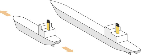
We’ll be concerned with two distinct types of scaling process: scaling in three dimensions, and scaling in one dimension only. Put simply, scaling in three dimensions means stretching the vehicle simultaneously along all three axes (length, width, and height) as shown in figure 2. All dimensions rise or fall in the same ratio so that the body retains its original shape, while the volume \(\nabla\) rises or falls in proportion to the cube of the vehicle’s length (and in fact \(\nabla\) is proportional to the cube of the linear distance \(d\) between any two reference points on the body surface). In the 1D process the body is scaled along its axial length (figure 3) while all other dimensions remain unchanged. Note that in 1D scaling, \(\nabla\) is proportional to the vehicle length \(l\) and vice versa.
Figure 2
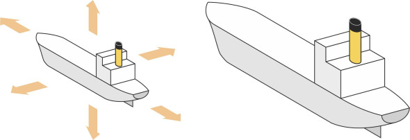
Figure 3
In the world of fluid mechanics, any problem that involves scaling a vehicle up or down in size raises an interesting question. What happens to the pattern of fluid flow around the vehicle – does it scale in the same ratio as the body size? As discussed in Section F1817, one can’t easily predict the change in lift and drag unless the original flow pattern and the scaled-up flow pattern are ‘similar’, with the spacing between the streamlines rising or falling in the same ratio as the vehicle body dimensions. This is guaranteed only if the parameters that characterise the fluid flow pattern are held constant. The parameters that will concern us here are the Reynolds number Re \(= Vd / \nu\) and the Froude number Fr \(= V / \sqrt{ g d}\), where \(d\) is some characteristic measure of vehicle size, usually its length, and \(\nu\) is the kinematic viscosity of the fluid. Given that the Reynolds number remains constant, the flow field around, for example, a sports car scales nicely and you can predict how the fluid forces exerted on the vehicle body will respond to a change in body size. In principle, if you want to scale it up in all 3 dimensions without changing the Reynolds number, you have to reduce the velocity in inverse proportion to \(d\) to preserve the original value of the quantity \(V d / \nu\). However, we want to gauge the effect of a size change independently of how fast the vehicle is moving, and prefer to keep V constant. This is why we are modelling the friction drag and the pressure drag separately.
Unfortunately the situation for ships is further complicated by the wave-making drag component, which hampers any attempt to assess the effects of changing \(d\) independently of velocity. In the case of aircraft, a different issue arises because the lift, drag and velocity are related in a unique way. We’ll postpone dealing with ships and aircraft until later.
Specific resistance
To recap, we are trying to find out how the total drag varies when we make a vehicle larger or smaller. It’s obvious that the larger the size of the vehicle, the more drag it will create, and equation 8 spells out the relationship between the two. What we really want to know is not whether it generates more drag, but whether it generates more drag in relation to its size. One way to answer this question is to work in terms of the specific resistance\(E\), defined as the ratio of drag \(D\) to gross weight \(W\), where \(D\) and \(W\) are expressed in the same units so that \(E\) emerges as a dimensionless ratio:
(9)
\[\begin{equation} E \quad =\quad \frac{D}{W} \end{equation}\]The concept of specific resistance was first proposed in 1950 by two aerodynamicists, Giuseppe Gabrielli and Theodore von Kármán [6]. It has since re-appeared in different forms [14]. In order to simplify matters later on, we’ll change the denominator from the weight of the vehicle to the weight of the equivalent volume of water, taking as our yardstick fresh water at \(4^{\circ}\)C. If we denote its mass density by \(\rho_w\), this weight comes to \(\nabla \rho_{w} g\), measured in force units. Then our volume-specific resistance \(E_{\nabla}\) or VSR for short, is given by:
(10)
\[\begin{equation} E_{\nabla} \quad = \quad \frac{D}{\nabla \rho_{w} g} \end{equation}\]which, like the specific resistance, is a dimensionless number. Note that the VSR is just \(S \times E\), where \(S\) is the specific gravity of the vehicle body. The fundamental idea, which is to measure drag in relation to the vehicle size, remains the same, but we are expressing ‘size’ in terms of volume rather than weight, which makes the results clearer and easier to interpret. In what follows we’ll try to work out how \(E_{\nabla}\) changes with \(\nabla\), separately for the 3D scaling process and the 1D scaling process.
Scaling in three dimensions
Since we’re deferring ships for special consideration later, we can for the time being drop the wave-making drag term from the right-hand side of equation 8. When scaling in three dimensions, we can drop the appendage drag term as well, which applies only to slender vehicles scaled in one dimension only. Assuming that the pressure drag scales in proportion to the cross-sectional area \(A\), and given that \(A\) is proportional to \(d^2\), or equivalently, proportional to \(\nabla^{2/3}\), it follows that \(D_{p}\) must scale as \(\nabla^{2/3}\). The situation with friction drag is less straightforward. If we scale the body in all three dimensions simultaneously, the two linear measurements \(b\) and \(l\) on the right hand side of equation 4 both scale in proportion to \(\nabla^{1/3}\), so \(D_{f}\) scales as \(\nabla^{1/3} \times \left( \nabla^{1/3} \right )^{4/5}\) or \(\nabla^{3/5}\). For reference, table 1 summarises the scaling relationships for pressure drag and friction drag.
| Drag component | How it scales with velocity V | How it scales with any linear measurement d | How it scales with volume displacement \(\nabla\) |
| Pressure drag \(D_p\) | \(V^2\) | \(d^2\) | \(\nabla^{2/3}\) |
| Friction drag \(D_f\) | \(V^{9/5}\) | \(d^{9/5}\) | \(\nabla^{3/5}\) |
Putting these two components together we arrive at the equation:
(11)
\[\begin{equation} D_{total} \quad = \quad D_{p} + D_{f} \quad = \quad k_{p} V^{2} \nabla^{2/3} + k_{f} V^{9/5} \nabla^{3/5} \end{equation}\]Now, the volume-specific resistance \(E_{\nabla}\) equals the total drag divided by \(\nabla \rho_{w} g\), hence
(12)
\[\begin{equation} E_{\nabla } \quad = \quad \frac{k_{p} V^{2} \nabla^{-1/3} + k_{f} V^{9/5}\nabla^{-{2/5}}}{\rho_{w} g} \end{equation}\]We can simplify things a little more if we fix \(V\) and focus solely on the effect of changing \(\nabla\), in which case equation 12 can be written:
(13)
\[\begin{equation} E_{\nabla} \quad = \quad c_{p} \nabla^{-1/3} + c_{f} \nabla^{-2/5} \end{equation}\]where \(c_p\) and \(c_f\) are constants. This is the result we are looking for, that the volume-specific resistance is a decreasing function of \(\nabla\). However, equation 13 doesn’t apply to ships and furthermore, it doesn’t apply to aircraft for the reason mentioned earlier, that for a machine that relies on aerodynamic lift for support, the speed and displacement are not independently scaleable. We’ll re-visit both these vehicle types separately later, but for now, we are left with a limited range of vehicle types to which equation 13 might apply. They include small cars and lighter-than air vehicles such as airships, and since they don’t produce wave-making drag, it also applies to submarines. For these vehicle types at least, provided you accept the assumptions made so far, and given a fixed cruising speed, both terms on the right hand side fall as the vehicle size increases. In this sense, a large submarine is hydrodynamically more efficient than a smaller one, having less resistance per unit volume of hull. The same applies to cars and to airships.
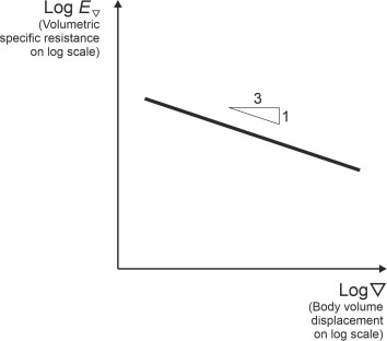
Before moving on, we can extract a little more information from equation 13. It relates to a special case: if the vehicle is sufficiently short and squat for the pressure drag to dominate, the friction drag term can be omitted and the right-hand side reduces to \(c_{p} \nabla^{-1/3}\). Clearly, the specific drag falls as the volume displacement rises, but by how much? As shown in figure 4, when both are plotted on a logarithmic scale, the graph of \(E_{\nabla}\) against \(\nabla\) is a straight line with slope -1/3. To make this more tangible, suppose you own two vehicles each of displacement \(\nabla\), and decide to replace them with a single vehicle of displacement \(2\nabla\). By definition, the specific drag changes from \(c_{p}\nabla^{-1/3}\) to \(c_{p} \left( 2\nabla \right)^{-1/3}\), and when you do the arithmetic, you’ll find this represents a fall of 20.6\(\%\) .
Figure 4
Scaling in one dimension only
Not all vehicles can be scaled up and down in three dimensions. For example, a passenger railway train can be stretched longitudinally, but the cross-section (the width and height of each coach) is essentially fixed by the layout of the track. The same applies to a heavy road truck. Consequently for one-dimensional scaling we have to re-work the specific drag formula. There are two main changes. First, the only dimension we can vary is the vehicle length \(l\) as measured in the direction of motion, so from here on we’ll use the symbol \(l\) to represent the scaling process rather than the more general quantity \(d\). The other dimensions such as width and height remain unchanged. Second, we now have four drag components rather than three, the additional component being the ‘appendage drag’ to which we referred earlier. As previously though, we’ll ignore the wave-making drag component and defer the consideration of ships until later.
In order to work out a revised version of equation 8 for the total drag, we’ll need first to determine how the pressure drag, friction drag, and appendage drag scale with \(\nabla\). The pressure drag \(D_p\) scales as the frontal area \(A\) and also as \(V^2\), but since the quantity \(A\) is now fixed, \(\nabla\) is not involved. In the case of the friction drag, since the perimeter \(b\) on the right hand side of equation 5 is now fixed, and noting that \(l\) is now proportional to \(\nabla\) (not \(\nabla^{1/3}\) as previously), it transpires that \(D_f\) scales as \(\nabla^{4/5}\) and is also proportional to \(V^{9/5}\) as before. Finally, the appendage drag is proportional to the number \(n\) of appendages. Assuming that the appendages are arranged at regular intervals along the vehicle body, it will scale as the vehicle length \(l\) and therefore as \(\nabla\); we’ll assume also that the drag for each appendage is proportional to \(V^2\). For reference, the scaling relationships for these three drag components are summarised in table 2.
| Drag component | How it scales with velocity V | How it scales with body length l | How it scales with volume displacement \(\nabla\) |
| Pressure drag \(D_p\) | \(V^2\) | Constant | Constant |
| Friction drag \(D_f\) | \(V^{9/5}\) | \(l^{4/5}\) | \(\nabla^{4/5}\) |
| Appendage drag \(D_a\) | \(V^2\) | \(l\) | \(\nabla\) |
Putting these three together we arrive at the equation:
(14)
\[\begin{eqnarray} D_{total} \quad & = & \quad D_{p} + D_{f} + D_{a}\nonumber \\ & = & \quad K_{p} V^{2} + K_{f} V^{9/5} \nabla^{4/5} + K_{a} V^{2} \nabla \end{eqnarray}\]where \(K_p\),\(K_f\), and \(K_a\) are constants. Proceeding as before, we derive an expression for the volume-specific resistance as follows:
(15)
\[\begin{eqnarray} E_{\nabla } \quad & = & \quad D_{total}/\left( \nabla \rho_{w} g \right)\nonumber \\ & = & \quad \left( K_{p} V^{2} \nabla^{-1} + K_{f} V^{9/5} \nabla^{-1/5} + K_{a} V^{2} \right) / \rho_{w} g \end{eqnarray}\]Let’s now fix \(V\) and focus solely on the effect of changing \(\nabla\), in which case equation 15 appears as:
(16)
\[\begin{equation} E_{\nabla } \quad = \quad C_{p} \nabla^{-1} + C_{f} \nabla^{-1/5} + C_{a} \end{equation}\]where \(C_p\), \(C_f\), \(C_a\) are constants. Again this is a decreasing function of \(\nabla\). Since we’re ruling out ships and aircraft for the moment, it applies only to railway trains and long road trucks, but for these vehicle types at least, it confirms that if you aim to carry a given payload over a given distance then in theory, a fleet of longer vehicles will consume less energy overcoming fluid resistance than a fleet of shorter vehicles having the same total volumetric carrying capacity.
Notice that if friction drag dominates, which is possible for long, narrow vehicles of this type, equation 16 reduces to
(17)
\[\begin{equation} E_{\nabla } \quad = \quad C_{f} \nabla^{-1/5} \end{equation}\]and after taking logs of both sides we get
(18)
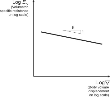
\[\begin{equation} \log {E_{\nabla }} \quad = \quad \log {C_f} - \frac{1}{5} \log \nabla \end{equation}\]so that as shown in figure 5, a plot of \(E_{\nabla}\) against \(\nabla\) using logarithmic scales on both axes will appear as a straight line with slope \(-1/5\). To make this concrete, suppose you own two vehicles each of displacement \(\nabla\), and replace them with a single vehicle of displacement \(2 \nabla\). Then the quantity \(E_{\nabla }\) changes from \(C_{p}\nabla^{-1/5}\) to \(C_{p} \left( 2 \nabla \right)^{-1/5}\), a relatively modest fall of \(12.9 \%\).
Figure 5
Results for different vehicle types
So far, we have derived two theoretical formulae for volume-specific resistance. Equation 13 deals with vehicles having a bluff shape that can be scaled up or down in three dimensions, while equation 16 deals with slender vehicles that we want to scale in one dimension only. Both point towards the conclusion that large vehicles are hydrodynamically more efficient than small ones, but the formulae apply only to land vehicles. For ships, we need additionally to take into account the wave-making drag, while for aircraft, we’ll need to take into account the resistance associated with creating lift. So let’s review the argument separately for each vehicle category.
Ships
Ships travel through water, which is a relatively dense fluid, much denser than air. Nevertheless, they encounter relatively little resistance per tonne of cargo carried. There are three reasons for this: first they move slowly, secondly, they don’t have to travel uphill, and thirdly they don’t encounter the mechanical forms of resistance such as rolling resistance that plague vehicles moving on land. But what does the data show - is there a consistent tendency for the volume-specific resistance to fall with increasing size? The answer seems to be yes. For yachts, the ratio of drag to weight displacement is inversely proportional to the square root of hull length [11], and data for other craft seems to suggest a similar relationship. In particular, the ratio for large, slow vessels tends to be quite small, in the region of 0.1 to 0.6 [9]. So we might expect the quantity we are working with – the volume-specific resistance \(E_\nabla\) – to fall with increasing size too.
In principle, a displacement vessel can be scaled in several different ways, but we’ll consider only the two alternatives mentioned earlier: (a) scaling in three dimensions, and (b) scaling in one dimension only, lengthways. Let’s start by assuming 3D scaling. In order to assess the effects for a displacement vessel such as a ship, we must re-visit equations equation 11 and equation 13, but with an additional term to allow for the wave-making resistance \(D_w\). For the moment, we’ll assume that \(D_w\) scales as an unknown function of \(V\) and \(\nabla\) as specified by equation 6, so we have
(19)
\[\begin{equation} D_{total} \quad = \quad D_{p} + D_{f} + D_{w} \quad = \quad k_{p} V^{2} \nabla ^{2/3} + k_{f} V^{9/5} \nabla^{3/5} + k_{w} f_{w} \left( V,\nabla \right) \end{equation}\](20)
\[\begin{equation} E_{\nabla } \quad = \quad \frac{ k_{p} V^{2} \nabla^{-1/3} + k_{f} V^{9/5} \nabla^{-2/5} + k_{w} \nabla^{-1} f_{w} \left( V,\nabla \right)}{ \rho_{w} g } \end{equation}\]Now we fix \(V\) and focus on the effect of changing \(\nabla\), writing equation 20 as:
(21)
\[\begin{equation} E_{\nabla } \quad = \quad c_{p} \nabla^{-1/3} + c_{f} \nabla^{-2/5} + c_{w} \nabla^{-1} f_{w} \left( V,\nabla \right) \end{equation}\]In equation 21, the first two terms on the right hand side – the resistance components that are associated with pressure drag and friction drag - are both decreasing functions of \(\nabla\), so the problem hinges on the behaviour of the third term: when this term is included, is the right hand side still a decreasing function of \(\nabla\)? It seems likely, for two reasons. First, this term contains a multiplying factor \(\nabla^{-1}\). Secondly, as explained in Section M1619, every ship has a ‘theoretical hull speed’, the maximum speed it can travel before the wave-making drag increases drastically and the vehicle starts to plane along the water surface. It is proportional to the square root of its length, so that other things being equal, large ships are faster than small ones, which in turn suggests that in general, larger ships incur less specific resistance.
But there is a possible snag. Unlike other types of resistance, wave-making drag varies with the speed and geometry of a displacement vessel in an unpredictable way because the bow and stern wave systems interfere with each other. The degree of interference depends on (a) how far the two wave systems are apart and (b) how fast the ship is travelling. Hence, as explained in Section M1620, there is no simple formula for estimating the value of the wave-making drag as a function of \(\nabla\) with \(V\) held constant. Its behaviour hinges on the Froude number \(V/\sqrt{gl}\) rather than the velocity as such; for example, faster displacement ships such as passenger liners operate at a Froude number around 0.35, which corresponds to a low resistance value that is sometimes called the ‘prismatic hollow’. Nevertheless, the overall trend is for the wavemaking resistance to rise with increasing Froude number and therefore to fall with increasing hull length \(l\). The rate of fall varies with \(l\) and locally may change sign, but given that in equation 21 the wavemaking resistance is multiplied by the factor \(\nabla^{-1}\), one might expect the third term on the right-hand side to be a decreasing function of \(\nabla\), so that the volume specific resistance falls with increasing size.
What about one-dimensional scaling? It is not unusual for an existing vessel to be cut in two and a new section inserted to increase its carrying capacity. Strictly speaking, a ship stretched in this way is not geometrically similar to the original because the leading and trailing sections (known as the ‘entrance’ and ‘run’) are not themselves stretched at all, so any results we derive for 1D scaling will only be approximate for a vessel treated in this way. Bearing this in mind, one can apply a process of reasoning similar to the one used for 3D scaling to show that although the friction element declines less rapidly in this case, the VSR for a ‘stretched’ vessel declines with increasing length too.
To conclude, hydrodynamic theory predicts that with either type of scaling, the volume-specific resistance falls as the size of the vessel increases. This assumes that the weight of the hull together with engines and ancillary equipment rises in proportion to the overall displacement \(\nabla\), whereas in reality it rises more quickly because of the way the stresses escalate with increasing size, and this has structural consequences to which we’ll return later.
Railway trains
Over the last few decades, journey speeds have risen dramatically for inter-city passenger trains, the only mode of transport that offers significantly faster travel than it did 50 years ago. Rolling resistance used to be important, but nowadays, when a train travels at 250 km/h or more, around 80\(\%\) of the overall resistance arises from aerodynamic drag [3] [7].
Compared with other mechanised vehicles, a railway train is long and narrow, so ideally, the whole formation of a passenger train – power cars and trailer cars - behaves aerodynamically like a javelin, albeit a javelin with notches cut into its sides together with protruberances at regular intervals along its length. Friction drag dominates [1] [3], with additional contributions from the appendage drag produced by turbulence around the bogies, current collectors and intakes for the air conditioning system. By comparison, the pressure drag is small, and the shape of the tail has little effect [10]. However, we’ll need to bear in mind that the flow field around a moving train is not as simple and straightforward as one might imagine. There’s usually a wind blowing at an angle to the track, and the motion of the ground as it passes underneath the vehicle disturbs the flow pattern, as does any trackside infrastructure passing alongside. It’s not easy to measure the resulting effect on drag or to investigate the pattern of air flow around the train in detail. One can attach probes to the body shell to measure the local fluid velocity, but wind tunnel tests are difficult: a model that is sufficiently large in cross-section to enable detailed investigations of, for example, the air flow around the bogies may be too long to fit into the tunnel. What we do know is that the boundary layer grows in thickness as it passes along the body surface and, having run out of kinetic energy, it separates at the rear (for the ETR 500 train mentioned in Section F1616, a quick calculation using the turbulent boundary layer model suggests that it is well over a metre thick at this point). Also, the airflow along the sides has an upward velocity component [1], rising and converging over the roof, and studies have revealed strong vortices in the wake of the rear trailing car [1] [2].
Here, we have taken into account only the pressure drag, friction drag and the appendage drag, so that the volume-specific resistance satisfies equation 15. It is a decreasing function of \(\nabla\), so if our assumptions are correct, then in terms of the drag per passenger seat, the aerodynamic efficiency of the train improves with increasing train length. However, the gain is not large. As stated earlier, if we ignore pressure drag and appendage drag, then doubling the train length yields a fall in VSR of only 13\(\%\).
Road vehicles
A heavy truck is like a railway train inasmuch as its height and width are fixed; only its length can change significantly. Since a long vehicle generates considerable drag through friction with the roof and side panels, one might expect the specific resistance profile to lie somewhere between that for a bluff body and a railway train. But in this case we can appeal to information from another source. Wind tunnel tests carried out on models during the 1960s showed that the drag coefficient \(C_D\) for a rectangular box rises with increasing length \(l\) towards an asymptote of the form
(22)
\[\begin{equation} C_D \quad \sim \quad c_{1} + c_{2} l \end{equation}\]where \(c_1\) and \(c_2\) are positive constants [8]. Their values depend on whether the front corners of the box are rounded, in which case the drag coefficient falls to a much lower value, but the functional form of equation 22 remains unchanged. Hence the drag for a long vehicle is given approximately by
(23)
\[\begin{equation} D \quad = \quad \frac{1}{2} \rho V^{2} A C_{D} \quad \sim \quad \frac{1}{2}\rho V^{2} A \left( c_{1} + c_{2} l \right) \end{equation}\]where \(A\) is the frontal area. Dividing both sides by \(\nabla \rho_{w} g\) gives us
(24)
\[\begin{equation} E_{\nabla } \quad = \quad \frac{D}{\nabla \rho_{w} g} \quad \sim \quad \frac{1}{2} \frac{\rho V^{2} A \left( c_{1} + {c}_{2} l \right)}{\nabla \rho_{w} g} \end{equation}\]Now, since \(A\) and \(\rho_w\) are fixed and \(l\) is proportional to \(\nabla\), we deduce that
(25)
\[\begin{equation} E_{\nabla } \quad = \quad c_{3} V^{2} \left(\nabla^{-1} + c_4 \right) \end{equation}\]where \(c_3\) and \(c_4\) are constants. Again, this is a decreasing function of \(\nabla\), which supports the hypothesis that like a railway train, a long truck is more aerodynamically efficient than a shorter one.
What about other road vehicles? A similar argument applies to buses, but not to automobiles, whose dimensions don’t scale up naturally in the same way. The roof height of a saloon car is governed largely by the seating posture of the occupants, and while luxury models are both longer and wider than entry-level models, they scale up in two dimensions rather than one. Nevertheless, from what we have learned so far we’d expect the larger models to have a lower drag coefficient, so it’s likely that in common with other vehicle types the VSR falls with increasing size. That doesn’t guarantee, of course, that the drag per passenger will fall if the owner of a modest family saloon trades up to a larger model and drives around with no-one else in the car!
Aircraft
Finally we turn to aircraft. Here, we are obliged to re-work the analysis, because the volume displacement \(\nabla\) of an aircraft and its velocity \(V\) are no longer independent - we can’t scale up the one without changing the other even if we wanted to. The reason is that when you increase the size of an aircraft, its weight rises more than the lift generated by its wings, and the aircraft must travel faster to stay aloft. To work out the implications, we’ll assume a 3D scaling process and take as our starting point the classical lift formula as set out originally in Section F1817, where the lift coefficient was assumed to be a function of the Reynolds number, the Froude number, and the Mach number. The Froude number applies only to ships, and since we’re dealing with subsonic aircraft only, Ma plays no part in the problem, and furthermore we’ll assume that the lift coefficient remains constant under changes in velocity and scale so we can omit the braces altogether:
(26)
\[\begin{equation} L \quad =\quad \frac{1}{2} \rho V^{2} A_{w} C_{L} \end{equation}\]where \(A_w\) denotes the wing area. This conveniently reduces to
(27)
\[\begin{equation} L \quad = \quad K_{1} V^{2} A_{w} \end{equation}\]where \(K_1\) is a constant. When cruising in level flight, the lift exactly balances the aircraft weight \(W\) so
(28)
\[\begin{equation} W \quad = \quad L \quad = \quad K_{1} V^{2} A_{w} \end{equation}\]In 3D scaling, the wing area is proportional to the square of the vehicle length or equivalently, proportional to \(\nabla^{2/3}\). After substituting this expression for \(A_w\) and re-arranging, equation 28 becomes:
(29)
\[\begin{equation} V^{2} \quad = \quad K_{2} W \nabla^{-2/3} \end{equation}\]where \(K_2\) is (yet another) constant. The next step involves a crucial assumption, that the weight of an aircraft rises in direct proportion to its volume. This is approximately true for nature’s ‘flying machines’ – birds and mammals capable of sustained flight with flapping wings. The average density of bone, muscle and other internal organs is roughly the same across a wide range of species, so that \(W\) scales as \(\nabla\) and vice versa. So after substituting a constant times \(W\) for \(\nabla\) on the right-hand side and taking square roots of both sides, equation 29 yields
(30)
\[\begin{equation} V \quad \propto \quad W^{1/6} \end{equation}\]This is the ‘one-sixth power law’, familiar to aeronautical engineers and also to biologists who are interested in bird flight [5] [12]. For the moment, let’s assume that the weight of an aircraft scales in the same way, directly in proportion to its volume, and work out what happens to the specific drag. We can re-write equation 30 as
(31)
\[\begin{equation} V \quad \propto \quad \nabla^{1/6} \end{equation}\]and now, if we substitute a constant times \(\nabla^{1/6}\) for \(V\) on the right-hand side of equation 12 and simplify, we get:
(32)
\[\begin{equation} E_{\nabla } \quad = \quad H_{p} + H_{f} \nabla^{-1/10} \end{equation}\]where \(H_p\) and \(H_f\) are constants. This is a decreasing function of \(\nabla\), but it decreases very slowly. Scaling an aircraft up in size has only a marginal effect, because a large aircraft must move faster to stay aloft, and as a result, it encounters greater drag purely because of its speed. Furthermore, as we’ll see in a moment, scaling up an aircraft introduces a weight penalty that we haven’t so far taken into account, so we can’t be certain that scaling up an aircraft will make it aerodynamically more efficient. All we can say is that by necessity, it must move faster: the cargo or passengers on board will reach their destinations more quickly, and the aircraft will be able to make more trips within a given time period. Economically, it may well be more productive.
Discussion
Our aim has been to investigate whether ‘big is beautiful’ in terms of hydrodynamic efficiency: do large vehicles generate less drag than small ones in relation to their cargo capacity? Subject to a number of assumptions, our theoretical model suggests this is true for land vehicles: the volume-specific resistance of a railway train or a road truck does indeed fall when the vehicle is scaled up in size. However, the case for ships and aircraft is more complicated.
The elephant effect
When a vehicle is scaled up in size, its structural framework must be strengthened to cope with the increased loads, each member being replaced with a thicker one. How much thicker should it be? Suppose the length of the vehicle is \(l\), say. A vehicle body is an assembly of struts, beams and panels designed to protect the occupants and maintain its shape regardless of the loads imposed on the structure during its lifetime. Assume we continue to use the same material; then if we scale up each component so that its dimensions (including length, breadth and thickness) increase in proportion to \(l\), its weight will increase in proportion to \(l^3\), and if we take only ‘static’ loading into account, the loads applied to it will increase in proportion to \(l^3\) too. But its cross-sectional area will scale only as \(l^2\), so the stress – the load per unit area - will rise. To keep all the stresses within their permissible limits, each member must be disproportionately thicker, with the inevitable consequence that the weight of the structure escalates more rapidly with increasing size than the volume. Biologists tell us that the radius of animal limbs scales as \(M^{3/8}\) whereas their length scales as \(M^{1/4}\) where \(M\) is body mass [13]. That’s why elephants look stocky compared with tigers: there is a limit to how large you can make anything before it collapses under its own weight.
This escalation has two distinct consequences. The first is that the structural members will take up a larger percentage of the total volume so that a proportion of the vehicle’s carrying capacity is lost. This somewhat undermines our concept of ‘hydrodynamic efficiency’: the resistance may fall in relation to the overall displacement \(\nabla\), but not necessarily in relation to the vehicle’s cargo-carrying capacity. The second is that the vehicle is heavier in relation to its size. You might think that weight is not an issue here, because the weight of a vehicle doesn’t affect its hydrodynamic behaviour. This might be true for land-based vehicles, but not for ships and aircraft. When fully loaded, a ship is designed to float with the gunwales at a safe distance above the water known as the ‘freeboard’. A little thought will show that in order to maintain a given ratio of freeboard to the overall depth of hull, the total weight of the vessel and its volume displacement must both increase in the same ratio when it is scaled up in size. So if the weight of the hull rises more quickly, the weight of cargo must be scaled at a reduced rate to compensate. The ‘elephant effect’ applies to aircraft too, so here too, the extra weight must be compensated somehow. There are two possible solutions: either (a) scale the cargo carrying capacity at a reduced rate, or (b) fly the aircraft faster, but in either case the VSR may no longer fall with increasing aircraft size.
So far we have assumed that the scaled-up vehicle is built using the same materials as the original. But it may be possible to mitigate the elephant effect by using lighter materials for critical parts of the structural framework. In recent years, marine architects have sometimes turned to aluminium rather than steel for smaller vessels - and additionally for the superstructure of passenger ships. For obvious reasons, aircraft designers have always put a high priority on lightweight materials so aluminium alloys are commonly in use, together with titanium alloys and carbon composites where the cost can be justified.
Are vehicles getting larger?
If large vehicles incur less resistance per unit of payload than smaller ones, you would expect vehicles generally to grow in size from one decade to the next. Less drag means less fuel. Of course, drag is not the only consideration, and for some vehicle types, it may not be particularly important. When investing in a vehicle fleet, a commercial operator will take into account track costs, maintenance costs, the cost of hiring the crew, and the capital costs including any financial risks associated with larger vehicles as compared to smaller ones. So what has actually happened? Let’s examine our four categories of transport vehicle in turn.
During the 19th and 20th centuries, ships grew steadily in length and displacement. Able to carry over half-a-million tonnes of crude oil, the largest tanker ever built was launched in 1979 under the name Knock Nevis. But she was scrapped in 2009, and no vessel of comparable displacement has appeared since. Meanwhile, container ships have continued to grow in in size. However, the operation of very large ships is constrained by external factors such as the width of the Panama Canal and the width of the Suez Canal, together with the availability of terminal facilities and maintenance facilities in dry dock.
Different factors apply to railway trains. During the last few decades, it has become possible to haul an extended goods train with several locomotives, all controlled by radio from a single cab, and in 1996 an Australian mining company ran a formation that was over 6 kilometers long [4]. However, trains of this size can’t operate on a passenger railway, where the number of coaches is determined by passenger demand and the length platform available at each station; most of the world’s passenger trains operate with between 8 and 12 coaches, and have done so for many years. By contrast, road vehicles have been growing in size slowly but steadily and the trend seems set to continue. There is now a possibility of linking heavy trucks together electronically for certain parts of the journey, which might yield a small fuel saving. Aircraft have been growing in size too, but the growth peaked around the turn of the century. In 2007 we saw the gargantuan Airbus 380 passenger jet enter service. In competition with the Boeing 747, it was intended to serve the ‘hub-and-spoke’ model of airline operations, carrying large passenger volumes between major airports, supported by feeder services provided by smaller aircraft to and from local ones. Airlines today are moving towards a ‘network’ model with direct flights between the origin and destination airports using smaller planes. Owing to modest sales, the Airbus company has announced that it will cease production of the A380 in 2021.
To conclude, after a long period in which the average size of almost every type of vehicle has increased steadily over time, it seems that for the time being at least, the trend has peaked. However the underlying problem will not go away, and to save fuel and reduce emissions, manufacturers are under pressure to reduce drag by any possible means. Eventually, we may stop worrying about whether the vehicles we use are sleek and aerodynamically efficient, but approach the problem in a more radical way. Should we turn instead to MAGLEV, or Elon Musk’s Hyperloop system, which generates hardly any resistance at all?