© US National Oceanic and Atmospheric Administration
M.1919
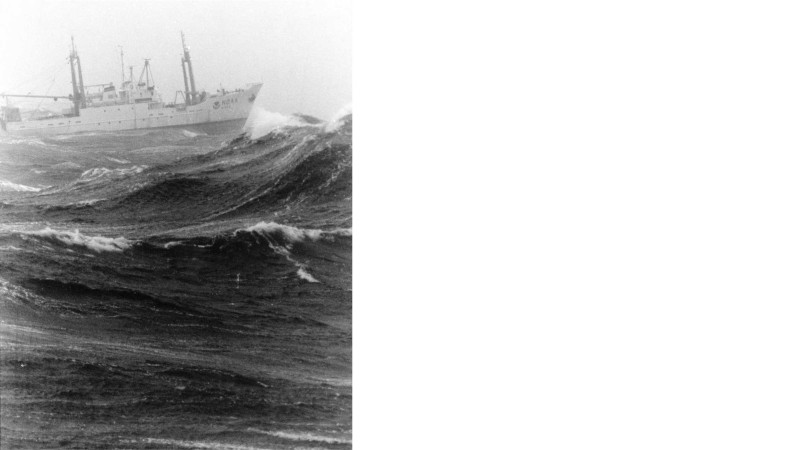
The marine environment
‘And the characteristic aspect of westerly weather … circumscribing the view of men, drenching their bodies, oppressing their souls, taking their breath away with booming gusts, deafening, blinding, driving, rushing them onwards in a swaying ship towards our coasts, lost in mists and rain.’
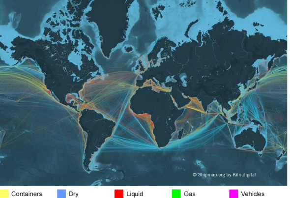
Over four thousand years ago, the people of Mesopotamia were experienced sailors. They imagined the oceans divided into ‘Seven Seas’, not the seven seas as we understand them today, but waters closer to the regions they knew. The phrase caught peoples’ imagination and has since been handed down across the generations. Nowadays we think of the seven seas as the Arctic, the North Atlantic, the South Atlantic, the Indian Ocean, the North Pacific, the South Pacific, and the Antarctic or Southern Ocean (figure 1). In reality they are all joined together – there is only one ‘sea’, and it covers over two thirds of our planet. The geography hasn’t changed but there is far more traffic, and the ships are making longer voyages. Their movements are logged: from the records of those that took place in the year 2012, the University College London Energy Institute has produced an animated display of the traffic world-wide on a projection of the globe, which you can download from its web site [18]. The results are shown in figure 2, in which the different coloured traces represent different kinds of ship: for example, blue represents dry bulk cargo ships while yellow represents container vessels. You might wonder why the traces aren’t spread out evenly across the globe. One reason is that the routes are linked to particular types of economic activity. Another is that sea conditions are favourable in some places and downright hostile in others. Finally, the oceans are themselves are moving, and not always in the direction the captain wants to go.
Figure 1
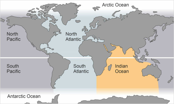
Figure 2
The sea in motion
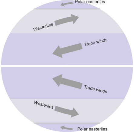
The oceans are moving because of the wind that blows across the water surface. In fact there are several winds that together make up a regular pattern, a series of belts around the earth’s circumference as shown in figure 3. There are six belts, and we’ll be looking at them more closely later, but for now, we’ll concentrate on the four nearest the equator. The bands immediately on either side blow from east to west and are commonly known as the Trade Winds because in past centuries, sailing ships relied on them all the year round: they enabled European explorers to reach America, and ultimately to travel around the globe. Further away from the equator, there are two more belts, one in the northern hemisphere and one in the southern hemisphere. They blow in the opposite direction from the Trade Winds, from west to east, and are often called the Westerlies.
Figure 3
Gyres
The winds create currents at the water surface, and whenever a current meets a land mass it is forced to turn north or south. The result is that in five of the seven major oceans, the water revolves like a vast, slowly moving whirlpool called a gyre. As shown in figure 4, the direction is clockwise in the northern hemisphere, while in the southern hemisphere, the direction is anti-clockwise. To explain the rotation, we’ll focus on one example: the north Atlantic.
Figure 4
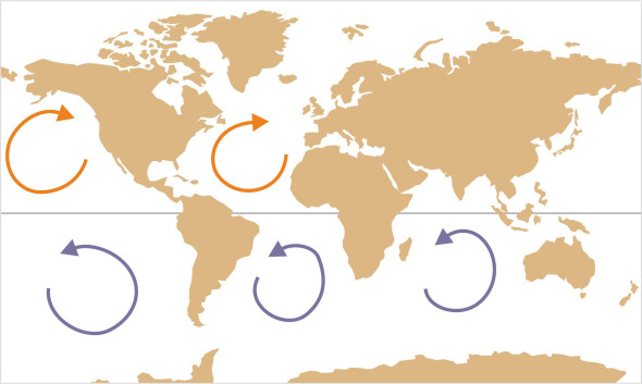
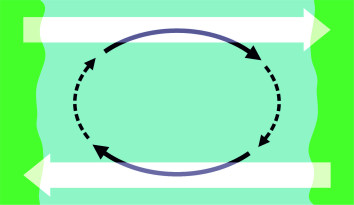
At high latitudes, the sea is driven towards the east, while closer to the equator, it is driven towards the west, in either case at a rate of a few kilometres per day. Since the two currents are moving in opposite directions, you might expect a degree of turbulence in between, with eddies forming at the interface. What actually happens is a more orderly kind of circulation, a gyre, and it’s brought about by the Coriolis effect. The earth itself is not stationary, but acts as a moving platform that when viewed from the north pole, rotates anticlockwise. In principle, any chunk of water in the north Atlantic is free to move in any direction on the platform surface, and when given an initial impetus, it will continue to move in a straight line relative to the distant stars. But as explained in Section F1818, as observed within the earth’s rotating frame of reference, it will veer to the right. This is a Coriolis acceleration, and it means that any random eddies will tend to form a coherent pattern of circulation around a common centre. Figure 5 shows how this circulation affects the oceans in the northern hemisphere. In the southern hemisphere the Coriolis acceleration acts in the opposite sense, so the South Atlantic, the South Pacific, and the Indian Ocean rotate anti-clockwise.
Figure 5
The major ocean currents
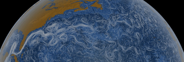
In reality the dynamics are more complicated. In some places the currents move upwards and downwards as well, carrying water masses at different temperatures to and from the ocean depths. But here, we’re more interested in what happens on the surface, where it turns out that the circulation is lop-sided. We’ll describe what happens in the north Atlantic first, starting with the current along its western perimeter. Moving within a narrow band, it reaches a speed of 5 knots as it leaves the Gulf of Mexico and squeezes northwards past the tip of Florida before heading across the North Atlantic carrying warm water towards Europe [1]. It’s called the Gulf Stream, and its path is traced out in the satellite picture shown in figure 6. When it reaches Europe, the current swerves gradually southwards and widens out. Notice that the current in figure 6 doesn’t follow a smooth curve as implied by the diagrammatic representation in figure 5, but is overlain with whorls and eddies – like the earth’s atmosphere, the sea has ‘weather’ too.
Figure 6
The pattern of circulation we have just described is similar for each of the five main oceans, and oceanographers have been able to replicate many of its features using mathematical models [15]. The most noticeable feature is the intense current along the western edge, which takes place in all the oceans north and south of the equator. The Kuroshio Current is the most concentrated sector of the north Pacific gyre, running northward along its western margin past Japan. Similarly, The Agulhas current runs southwards along the east coast of Africa. All three of these currents average around 2-3 knots, which can significantly affect the journey time for vessels sailing on local routes. We can explain these currents partly as a consequence of the Coriolis effect (other factors are involved, but they are beyond our scope here). Suppose we set up a shallow tray of water on a rotating platform, and allow the water to settle down so it rotates as the same speed as the tray. If we choose a particular chunk of water and propel it in a particular direction, it will veer to the right. The curvature of its path is measured by the Coriolis acceleration, which we’ll denote by \(a_{Cor}\). Its value is proportional to the rate of rotation \(\omega\) of the platform and the velocity \(v\) of the chunk relative to that platform [3], specifically:
(1)
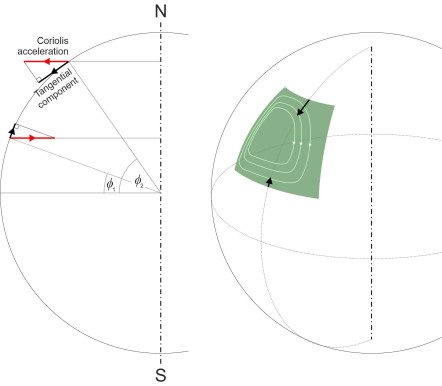
\[\begin{equation} a_{Cor} \quad = \quad 2 \omega v \end{equation}\]Now transfer the problem on a larger scale to the north Atlantic Ocean, where the Trade wind propels the current along its southern perimeter towards the west at velocity \(v\). If we denote the earth’s rate of rotation by \(\omega\), we can apply a similar formula to predict the Coriolis acceleration that causes the water current to veer to the right. However, there is a difference: the Coriolis acceleration predicted by equation 1 applies to movement on a flat tray at right angles to the axis of rotation. But the earth is spherical, and the oceans are tilted relative to its axis of rotation. As will be apparent from figure 7, for a point at latitude \(\phi_1\), say, the acceleration component that matters - the one tangential to the ocean surface - is actually somewhat less, \(2 \omega v \sin \phi_1\). The southern edge of the gyre in the north Atlantic Ocean occurs at a latitude of roughly \(25^{\circ}\) north, and at this latitude, the Coriolis acceleration is \(2 \omega v \times \sin 25^{\circ} = 0.845\omega v\) approximately. But the northern edge occurs at a latitude \(\phi_2\) of around \(50^{\circ}\), and here, the Coriolis acceleration is \(2 \omega v \times \sin 50^{\circ} = 1.532 \omega v\), which is almost twice as large. Hence the tendency to veer to the right is smaller along the southern perimeter of the gyre. So if we trace the current along this southern perimeter, we see it run up against the east coast of the USA, where it is deflected sharply to the north in a concentrated stream that we call the Gulf Stream. By contrast, along the northern perimeter, the acceleration is greater, and the Gulf Stream veers to the right as it approaches northern Europe, and spreads out over a wide area.
Figure 7
Tides
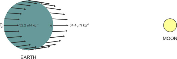
Oceans move in another way too, a motion that’s familiar to everyone: the regular ebb and flow of the tide. The moon provides the main driving force, which acts through two distinct mechanisms. The first is the moon’s gravitational pull, whose effect is easier to understand if we ignore the fact that the earth is spinning, and imagine instead that both the earth and the moon are held in fixed positions, frozen in space as it were. Like any astronomical body, the moon exerts a gravitional pull on anything nearby. Figure 8 shows the force acting on a one-kilogram mass of water positioned on different parts of the earth’s surface. At the point P1 closest to the moon, the pull works out at approximately \(34.4\ \mu \text{N kg}^{-1}\) (this is a very small force, measured in units of micronewtons per kilogram of water, or a millionth of a newton per kilogram). At a point P2 on the ‘far side’ of the earth which is a little further away, the force is slightly weaker, around \(32.2\ \mu \text{N kg}^{-1}\).
Figure 8
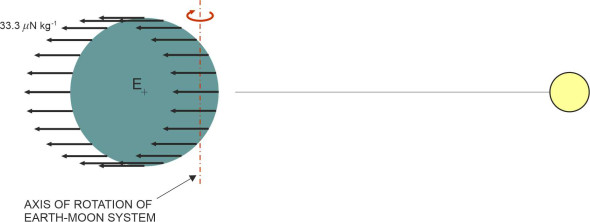
The second force mechanism arises from the rotation of the earth-moon gravitational system, which undergoes a complete revolution every 27.3 days. The centre of mass of the system lies inside the earth at a distance of 4600 km from its centre. The earth is not stationary, but like the moon, orbits round this centre of mass, so both the earth and the moon undergo centrifugal forces. For reasons explained in the Appendix to this Section, the earth’s centrifugal force has the same numerical value and acts in the same direction at all points on the earth’s surface and at all points within the interior, as shown in figure 9. It amounts to approximately \(33.3\ \mu \text{N kg}^{-1}\) and is aligned in the direction away from the moon and parallel to the straight line that joins the moon with the earth’s centre E.
Figure 9
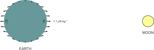
Finally, figure 10 shows what happens when the centrifugal and gravitational forces are added together. We find that the resultant force at P1 has a value of roughly \(1\ \mu \text{N kg}^{-1}\). It acts vertically upwards and has a negligible effect on the water level. In the surrounding region, the force diminishes gradually with distance but it is directed at an angle to the vertical and therefore has a horizontal component. It’s this horizontal component that causes water particles to flow tangentially towards P1 in sufficient volume to raise the level by about 600 mm and create a ‘bulge’ in the water surface on the near side of the planet. On the far side of the earth at P2, the resultant force acts in the opposite direction, away from the moon, because the centrifugal force dominates the gravitational pull. As explained in the Appendix, the resultant force is slightly smaller than its counterpart at P1; the tangential forces in the surrounding area are reduced accordingly, so the far-side bulge is slightly less pronounced.
Figure 10
Now for the final step. Within the rotating gravitational system, the earth itself is spinning relative to the moon, making a complete revolution every 24 hours and 50 minutes plus a few seconds. The oceans spin with it, but the bulges don’t. We can imagine them effectively tied to the moon’s location, so that each meridian on the earth’s surface passes through both bulges during a single revolution. As seen from the earth’s frame of reference, we now have two bulges that sweep round the globe in the form of two tidal waves with an interval of about 12 hours and 25 minutes between them. Since the earth’s surface at the equator is rotating at a tangential velocity of 1608 km/h (just under 1000 mph) relative to the moon, the tidal bulges skate across the ocean at supersonic speed. But the water particles themselves are moving quite slowly – it’s the geometry that’s supersonic. Since the height of each bulge is less than a metre in mid-ocean, and since it takes many hours for the ‘crest’ to pass by, we don’t notice it.
More important is the fact that the waves are ‘forced’ waves. The average depth of the oceans is less than 4 000 m, which means that very long waves like the tidal bulges are travelling effectively in shallow water, and each bulge lags behind the motion of the moon, typically by an hour or two. This time lag is not represented in any of the diagrams shown here. But crucially, the oceans are divided by land masses that get in the way, so the bulges don’t move as freely as our model might suggest. When a bulge reaches a shoreline, it will pile up like water sloshing from side to side in a bowl, and if we look at matters more closely, we see that the pattern of movement varies from one ocean basin to the next, according to its size and shape.
For less extensive bodies of water such as Mediterranean the tidal range is small, while in other cases such as the Atlantic Ocean, the range is larger. In some places, a bulge must thread its way through a narrow gap or around a peninsula to a wider ocean beyond, and this can delay the peak tide. In the North Sea and Baltic Sea, the delay can be as much as two days. In addition, the flow is influenced by Coriolis forces, so that within four of the seven seas, the tide rotates around the basin, visiting all points around the circumference in turn. This doesn’t apply to the Western Pacific, the South Atlantic, or the Antarctic Ocean, none of which is bounded by a land mass to the west [17].
At a more local level, irregularities in the coastline can have dramatic effects. For example, within a sharp indentation such as a river estuary, the incoming tide will pile up as it funnels into an increasingly narrow space. The effect works in reverse when the tide falls, and the result is a greatly increased tidal range, in some cases of the order of 15 metres, as happens around parts of northern Canada and also the UK. Then there are meteorological factors that alter the pattern on a daily basis, including variations in atmospheric pressure and wind that can trigger ‘surges’ well above the predicted level.
Also, we have greatly simplified matters because we haven’t taken the sun’s influence into account. In practice therefore, the gravitational model described here can’t predict the tides for any real location – it’s just the starting point for more sophisticated methods that you can find described in, for example [20]. The predictions are generated by computer using statistical models fitted to local data that has accumulated from tide gauge measurements over many decades, and the results are kept under constant review. Each model predicts the tidal elevation as the sum of many sinusoidal wave forms whose periods are derived from the motions of the earth, the moon and the sun. The results are published by navigational authorities such as the US National Oceanic and Atmospheric Administration NOAA and the UK Hydrographic Office, and you can find them on the web sites listed under Further Reading at the end of this Section [21] [22]. So at this point, we’ll put the matter aside and turn instead to another element in the marine environment that is equally if not more important.
Wind
Wherever you live, you will see changes in the weather from day to day. The changes are caused by movement of the earth’s atmosphere. The movement is driven by the energy of the sun, which creates local temperature differences and variations in air density that in turn give rise to currents of air with greater or lesser moisture content. As a result, we see winds, clouds and rain. Some weather patterns extend over a large area, while others are more localised. Within limits, their evolution can be predicted, and the predictions are vital for people whose livelihood depends on good weather, especially mariners.
Wind strength
In the past, seafarers used to measure the strength of the wind on a subjective scale. Based on the work of several predecessors, it was devised by Francis Beaufort, an officer in the UK Royal Navy. The Navy adopted the scale in 1830 and it was first used on the voyage of the Beagle. Among the passengers was Charles Darwin, whose studies during the voyage led to his celebrated theory of evolution. At the time, the Beaufort scale described the wind in terms of its effects on the sails of a typical frigate of the kind that was built during the early nineteenth century, but in later years it was modified and extended. Nowadays the scale is combined with numerical wind speeds that provide a more objective basis for measurement.
| Number | Description | Speed at 10 m above sea level (knots) | Mid-range of speeds, (m/s) |
|---|---|---|---|
| 0 | Calm | Less than 1 | 0.0 |
| 1 | Light air | 1 – 3 | 0.8 |
| 2 | Light breeze | 4 – 6 | 2.4 |
| 3 | Gentle breeze | 7 – 10 | 4.3 |
| 4 | Moderate breeze | 11 – 16 | 6.7 |
| 5 | Fresh breeze | 17 – 21 | 9.3 |
| 6 | Strong breeze | 22 – 27 | 12.3 |
| 7 | Moderate gale | 28 – 33 | 15.5 |
| 8 | Fresh gale | 34 – 40 | 18.9 |
| 9 | Strong gale | 41 – 47 | 22.6 |
| 10 | Whole gale | 48 – 55 | 26.4 |
| 11 | Storm | 56 – 64 | 30.5 |
| 12 | Hurricane | 65 – 71 | - |
Strictly speaking, the wind speeds refer to conditions at a height of 10 m above sea level (below that level, the speeds fall owing to friction with the water surface [14]). The strongest winds are associated with circulating bodies of air known as hurricanes and typhoons. Their formation is described in Section F1818.
Aerodynamic forces
Among other things, the wind creates waves that can damage a ship and threaten the safety of those on board. We’ll be looking at waves shortly. First, let’s examine the pressure that the flow of air exerts directly on the hull. During a storm, the pressure can reach 500 N/m2 [13]. It’s small compared with the impact pressure of a water wave, but when viewed from the side, the surface area of an empty cargo ship may amount to a thousand square metres. A storm force wind can exert a force of 500 kN on an area of this size, enough to make the ship heel, and make rolling motions signicantly more dangerous in a beam sea. It can also play tricks with the smoke exhaust from a ship’s funnel, and on a passenger ship, you don’t want the plume to envelope the passengers at deck level [14].
What about a headwind? As noted in Section M1619, in calm conditions, the air resistance of a modern ship typically accounts for between 2% and 4% of the total resistance to motion, a relatively small amount. However, the situation changes in a headwind, which raises the speed of the air flowing over the hull and superstructure. Since aerodynamic forces generally are proportional to the square of the wind velocity, the air resistance may become significant. Recently, interest has focussed on the aerodynamics of container ships, whose air resistance when loaded is relatively high, particularly in an oblique headwind.
How the wind makes waves
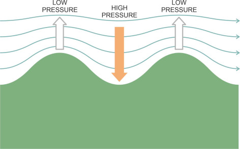
When we look at the ocean, our attention is drawn to the continual, restless movement of the waves. Almost all of them are caused by the wind. It’s not immediately obvious how the process works. How can an air current that is moving horizontally across the water surface cause peaks to rise vertically above the still water level? The problem has intrigued scientists for at least 200 years and still hasn’t been completely resolved. In a very readable book devoted to ocean waves [24], Professor Jack B Zirker has set out the story so far. Let’s look at one possible explanation. It starts with the notion that a surface wave is not a passive object. Once created, it will disturb the wind that creates it – the two interact. Since no ocean surface is completely smooth, any irregularity, however small, will trigger the interaction. Imagine a slightly raised area of water, which for sake of argument we’ll call a micro-crest. Initially, the micro-crest will be tiny, but it still represents an obstruction that squeezes the streamlines together so that the air speeds up a little as it rises over the top, like the air passing over an aircraft wing. In conformity with Bernoulli’s Law, the pressure will fall, and the reduced pressure will draw more water to pile on top of the micro-crest, producing a further increase in height as shown in figure 11. The increased height will lead to a further reduction in pressure and so on – the effect is self-reinforcing. So in a mathematical sense, the water surface is unstable [5] – it is hard for waves not to form.
Figure 11
However, it was discovered many years ago that the forces produced in this way are too small to explain the rate of growth of waves that we see in everyday life. A further mechanism is needed, and one possible candidate is resonance. When passing over a rough surface, a current of air will form eddies over the peaks. The eddies are cylinders of air like logs rolling down a hillside, each rotating about a horizontal axis. It is possible for the frequency of eddies to fall into resonance with the waves on the water surface and thereby boost the rate of energy transfer. We also know that waves can exchange energy among themselves when they collide, and it seems that under precisely defined conditions, the larger waves in a group will draw energy from those of shorter wavelength, gaining speed while growing to an appreciable size. In the next Section (M1820) we’ll examine waves more closely, in particular, how they form, their shapes, and how they move across the water surface. In deep water, the wave pattern may be quite complicated, with several distinct wave trains superimposed on top of one another where their paths cross. But provided their amplitudes are not too large, for each component, the phase velocity and wavelength are related by the formula:
(2)
\[\begin{equation} V \quad = \quad \sqrt{\frac{g \lambda}{2 \pi}} \end{equation}\]Coast
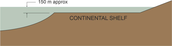
For passengers who’ve been at sea for a while, it’s reassuring to see land on the horizon. But the crew will be alert, because close to land, a ship is not necessarily safer than it would be in deep water. Much of the earth’s land mass has been eroded over thousands of years and the resulting sediment has accumulated in a strip along the shoreline that varies from zero to several hundred kilometres in width. It is known as the Continental Shelf (figure 12). It is here, where the water is less than 200 m deep, that a ship is most likely to be wrecked: either pierced by rocks hidden below the surface, or stranded at low tide. The risk escalates when the wind is blowing onshore. If the engines break down or the rudder fails, the ship must anchor. Otherwise, it will be skewered in position and pounded by waves until the hull eventually disintegrates. Before steam power arrived during the 19th century, roughly 1000 vessels per year were lost around the shores of Britain alone, so that today there are estimated to be 250 000 wrecks scattered on the seabed [23]. Nowadays such instances are rare, but nevertheless, it’s interesting to observe how conditions change as a ship approaches the end of its voyage.
Figure 12
Shoaling
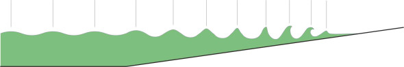
In the next Section, we’ll see that in open water, the waves form a chaotic jumble, but their behaviour changes as they enter shallow water. Magically almost, the jumble turns into a more orderly sequence of waves that grow in height and definition before they break on shore. What is going on here? Three aspects seem to call for explanation: (i) the growth in wave height, (ii) the appearance of a regular pattern, and (iii) the collapse of the wave crests. The growth in height can be explained by the dynamics of wave motion in shallow water. The relationship between phase velocity and wavelength changes to:
(3)
\[\begin{equation} V \quad = \quad \sqrt{\frac{g \lambda}{2 \pi} \tanh \left( \frac{2 \pi h}{\lambda} \right) } \end{equation}\]which is identical to equation 2 except for the factor \(\tanh (2 \pi h/ \lambda)\) under the square root sign. Since the hyperbolic tangent of any finite real number is always less than 1, the phase velocity of a wave is always reduced when it enters shallow water, and moreover it continues to fall as the depth diminishes [11]. Now, the frequency of a wave train is measured by the number of crests passing a given point per unit time. Its value must remain unchanged as they approach the shore, otherwise some of the waves would have to disappear, or new ones appear from nowhere. And since by definition the wavelength is equal to the phase velocity divided by the frequency, if the velocity falls the wavelength must fall too: the waves are squashed in the direction of motion. However, the energy contained within a wave per unit surface area is proportional to the square of its height [8]. This energy remains more-or-less unchanged as the wave approaches the shore. Since the surface area per wave decreases when the wavelength falls, the height must grow.
Now for the regular pattern. When the wave height reaches a value of the same order as the average depth of water, there is another critical change. The individual wave trains that ride over one another at different speeds in deeper water lose their identity because in shallow water, all waves travel at the same speed, whose numerical value is equal to \(\sqrt{gd}\) where \(d\) is the water depth. Waves travelling in the same direction at similar speeds tend to coalesce, so consecutive crests arrive at more regular intervals.
Finally, we turn to the point where the wave crests topple over onto the beach. Here we need to look beneath the wave crest to see what is happening. The fluid particles no longer follow a circular orbit as they might in deep water – instead, the circles are squashed into ellipses [2]. The ellipses are stretched horizontally, which means that particles at the bottom oscillate back and forth in straight lines (figure 13), a movement that generates friction with the seabed. People often suppose that it’s the friction that causes the waves to break, but the phenomenon can be explained even if no friction is present. Each particle inside the wave is moving in an elliptical orbit, and when carried up into the peak, momentarily it travels in the same direction as the wave itself. As the water gets shallower, the phase velocity falls, eventually falling below the forward speed of the particles in the upper crest. At this point, the crest is moving faster than the main body of the wave [9]. Hence the wave becomes unstable and it collapses [12] [6]. The sequence is shown diagrammatically in figure 14.
Figure 13
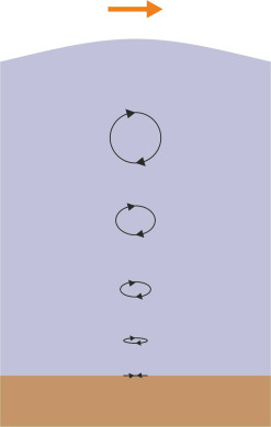
Figure 14
The cross-section of a breaking wave can take on one of several distinct forms: spilling, collapsing, surging and plunging. Of these, the last is the most spectacular form. In a plunging wave, the crest curls over and seems to hang momentarily in mid-air before crashing onto the trough below. Modelling its behaviour involves a specific branch of hydrodynamics called stream function theory, a topic that we won’t pursue here. But it’s worth mentioning that if a plunging wave collides with a solid barrier, the air trapped beneath the crest is compressed and then propelled upwards with explosive force, carrying a significant volume of spray high into the air; it was ‘swash’ created in this manner that broke over the sea defences and flooded several towns along the Thames Estuary in 1953, resulting in the loss of many lives. Equally, a plunging wave is the kind most feared by seafarers, because of its potential impact on a ship’s hull.
Wave refraction
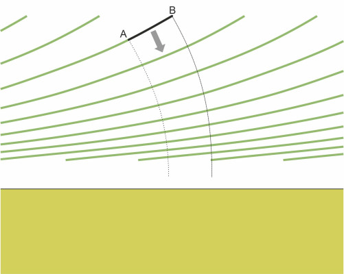
The fact that waves slow down in shallow water explains why waves that are travelling at an angle to the coast tend to turn towards the shoreline. They are refracted in the same way as light when it moves from a less dense medium to a denser one. In figure 15, the wave crest AB is shown with the point A nearer the shoreline and point B further away. As point A approaches shallow water, it slows down, while point B, together with all points between, doesn’t slow down as much. Like a troop of soldiers ‘wheeling’ on the parade ground, the wave swings round until it arrives parallel – or almost parallel - to the shore.
Figure 15
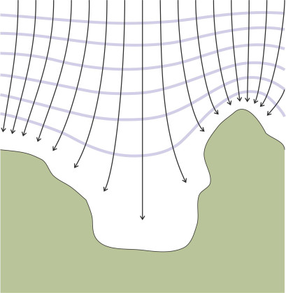
This refraction has interesting consequences for ships. It means that an indentation in the coastline as shown in figure 16 will cause the incoming waves to spread out so their energy is dispersed along a greater length of beach than would otherwise be the case. This is why a coastal bay offers a safe anchorage where the wave action is reduced compared with other locations nearby. A bay is a natural haven [6]. Conversely, a promontory will attract waves, causing them to focus their energy so that a ship sailing close by will experience a greater buffeting.
Figure 16
An emerging problem
In this Section we have viewed the sea as a hostile environment in which storms damage ships and injure the people who sail in them. We haven’t mentioned the obverse, that is to say, how ships can damage the marine environment. In the past, it didn’t seem to be a problem. Vast, remote and largely unexplored, the sea could withstand almost any degree of interference. We now know this isn’t true: a growing body of research has revealed how human activities are changing the ocean environment. Here, we’re concerned specifically with the damage caused by shipping. It’s a specialist field and we won’t go into detail, but it’s worth listing some areas of concern as set out in [7]:
- Discharges into the water: wastewater including sewage, oil spills, ‘operational’ discharges of dry bulk cargo such as coal and minerals, water from exhaust gas scrubber systems, litter including plastic debris (mainly from fishing nets), toxic particles of anti-fouling paint, and potentially invasive species discharged in ballast water in overseas ports.
- Physical impacts: sub-surface noise, artificial light, collisions with sea creatures, shoreline erosion, stirring of sediments on the seabed, and abandoned shipwrecks.
- Air emissions: carbon dioxide CO2 and other greenhouse gases, sulphur dioxide SO2, nitrogen oxides NO\(_\text{x}\), particulate matter, volatile organic compounds, and gases that remove ozone from the upper atmosphere such as halocarbons and HCFC refrigerants.
Not all of these are significant problems. But the volume of shipping has risen dramatically in recent decades, and many observers are concerned that shipping is not regulated in the same way as other branches of the transport industry. Ships move in places where they can’t easily be observed, and there is very little data about what is happening. You’ll find brief remarks on some of the issues in this web site, for example noise and vibration caused by ships’ propellers (Sections M1410 and M1405). Given the contribution of diesel fuel to climate change together with rising underwater noise levels, the growing quantity of chemicals transported by sea, and the transfer of potentially invasive species, there is a growing case for action on an international scale.
Appendix: The tidal forcing mechanism
The moon exerts a gravitional pull on the oceans in the same way that it exerts a gravitational pull on the earth itself. Take, for example, a small chunk of water that lies at a particular point P1, the part of the earth closest to the moon as shown in figure 8. Newton’s Law of Gravitation tells us that the gravitational attraction \(F_G\) between a body of mass \(M_1\) and a second body of mass \(M_2\) is given by
(4)
\[\begin{equation} F_{G} \quad = \frac{G M_{1} M_{2}}{D^2} \end{equation}\]where \(D\) is the distance between the two bodies (measured as the distance between their centres of mass), and \(G\) is the gravitational constant, whose value has been determined experimentally at \(6.674 \times 10^{-11} \text{ N m}^2 \text{ kg}^{-2}\). Suppose our chunk of water weighs one kilogram. Then it will be pulled vertically upwards by a force of magnitude
(5)
\[\begin{equation} F_{1G} \quad = \frac{G M_{moon} \times 1}{(d-r)^2} \end{equation}\]where \(M_{moon}\) denotes the mass of the moon, \(r\) is the radius of the earth at point P1, and \(d\) is the distance between the centre of the earth and the centre of moon. The force works out at approximately \(34.4 \ \mu \text{N kg}^{-1}\). Similarly, at point P2 on the ‘far side’ of the earth, the force acting on a 1 kg chunk of seawater is given by
(6)
\[\begin{equation} F_{2G} \quad = \frac{G M_{moon}}{(d+r)^2} \end{equation}\]which works out at \(32.2 \ \mu \text{N kg}^{-1}\). Here, the force is slightly weaker, and it draws the water downwards not upwards.
The second force mechanism arises from the rotation of the earth-moon gravitational system, which completes a revolution every 27.3 days. To picture the outcome, we’ll allow the earth to shift within the plane of the moon’s orbit, but not to rotate relative to the distant stars. The centre of mass of the system lies inside the earth at a distance of 4600 km (around three-quarters of the earth’s radius) from its centre. The earth is not stationary, but travels in a very small circle around the common centre of mass. The radius \(R_E\) of its orbit is given by
(7)
\[\begin{equation} R_E \quad = \quad \frac{M_{moon} d}{M_{earth}+M_{moon}} \end{equation}\]Since the earth is not spinning on its axis, each point on its surface (and indeed each point within the interior) follows a similar orbit. Although each orbit has a different centre, it will have the same radius \(R_E\). The centrifugal force \(F\) acting on a body of mass \(M\) that follows a circular orbit of radius \(R\) with an angular velocity \(\omega\) is given by
(8)
\[\begin{equation} \text{Centrifugal force} \quad = \quad M R \omega^2 \end{equation}\]For our chunk of seawater, \(M = 1\) kg, and regardless of where it is located, the centrifugal force will have the same value \(F_C\) given by
(9)
\[\begin{equation} F_{C} \quad = \quad R_{E} \omega^2 \end{equation}\]Knowing the period of revolution of the earth-moon system, in principle we can work out its angular velocity \(\omega\), which is \(2 \pi \tau\) where \(\tau\) is the period in seconds, and substitute the result into the right-hand side of equation 9 together with the value of \(R_E\) calculated from equation 7 to arrive at a figure for \(F_C\). We can then work out the resultant force for any particle on the earth’s surface by subtracting the centrifugal force from the gravitational attraction. However, there is a snag. The resultant force is a relatively small number that emerges as the difference between two large ones, and any error or ambiguity in the data leads to a large error in the outcome. And there are indeed ambiguities: for example, the moon’s orbit is not precisely circular, and because the formulae embodied in equations equation 5, equation 6 and equation 9 overlook this, the estimates of \(F_{1G}\) and \(F_{2G}\) are not strictly comparable with the estimate of \(F_C\).
We can avoid this problem by noticing that the gravitational forces and the centrifugal force are related: at the earth’s centre E, the gravitational attraction \(F_{GE}\) and the centrifugal force \(F_C\) are equal and opposite, so the resultant force \(F_E\) is zero. We can therefore put
(10)
\[\begin{equation} F_{E} \quad = \quad \frac{G M_{moon}}{d^2} - R_{E} \omega^2 \quad = \quad 0 \end{equation}\]Now we can substitute \(M_{moon} G / d^2\) for \(R_{E} \omega^2\) on the right-hand side of equation 9 to get a consistent estimate of the centrifugal force, which comes to approximately \(33.3\ \mu \text{N kg}^{-1}\). Hence the resultant force on the ‘nearside’ bulge is \(34.4 - 33.3 = 1.1\ \mu \text{N kg}^{-1}\) upwards, towards the moon. On the far side, the resultant force lies in the opposite direction, with a roughly equal magnitude of around \(1.1 \ \mu \text{N kg}^{-1}\) away from the moon: the two tidal bulges are driven by approximately equal forces. They’re never exactly equal, but if you want to go further you can expand equations equation 5 and equation 6 as binomial series, and show that as the ratio \(r/d\) tends to zero, the near-side and far-side forces converge asymptotically on the same value. Furthermore, the values of the forces themselves diminish asymptotically to zero, illustrating an interesting fact – the tidal forces arise not from the gravitational pull of the moon as such, but the difference in pull acting on the near and far sides of the planet.
Acknowledgements
The photo on the opening page shows the US National Oceanic and Atmospheric Administration ship Delaware II in rough weather on Georges Bank off the coast of New England on the eastern seaboard of the USA (photo by National Oceanic and Atmospheric Administration, US Department of Commerce, available at http://www.photolib.noaa.gov/bigs/wea00810.jpg, Public Domain, accessed 4 January 2017).
Figure 2 based on Map of ship movements world wide in 2012, University College London Energy Institute, graphics by Kiln, available at http://www.informationisbeautifulawards.com/showcase/1580-shipmap-org (accessed 12 May 2021).
Figure 6: NASA Scientific Visualisation Studio, Gulf Stream sea surface currents and temperatures, image available at: https://svs.gsfc.nasa.gov/3913 (accessed 12 May 2021).