© Penny Wright
C.1508
Arranging the wheels
Towards the end of the nineteenth century, the motor car evolved through many configurations before settling on the one with which we are familiar today. Some of the early machines now seem outlandish. Inventors were unsure how many wheels a vehicle needed, where and how they should be attached, and how the vehicle should be steered. The engine, wheels, and passenger seats were arranged in different ways until the industry finally arrived at common format with the passenger compartment at the rear and the engine at the front driving the rear wheels. There has been little change since then except for a shift to front wheel drive. But is there no better layout?
How many?
The question can be broken down into two parts: (a) the number of wheels and (b) how they are arranged around the vehicle body. We’ll deal with the number question first. Almost all cars have four wheels, but why not six, or three? A hundred years ago, the case for lots of wheels was perhaps more obvious than it is today: the roads were bumpy and we might imagine that in some sense, multiple axles ‘take the average’ of a rough road surface to give a smoother ride.
Figure 1
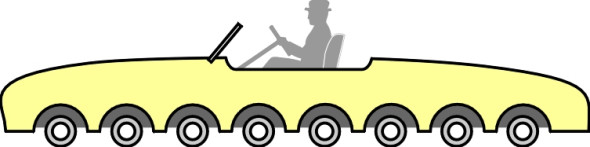
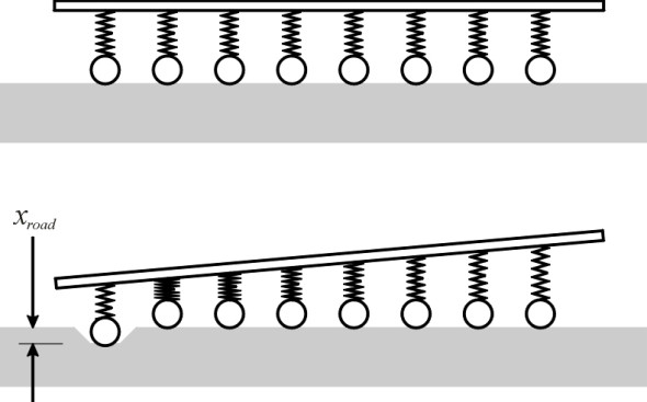
Let us frame this idea more precisely. Suppose a vehicle has n equally spaced axles as shown in figure 1. To keep things simple we’ll suppose that the driver sits at the midpoint, and the suspension characteristics are uniform across all the axles. The vehicle moves slowly along a flat horizontal surface until it arrives at a trough lying at right angles across its path. The leading axle rolls into the trough; this represents input from the road surface (figure 2). But the trough is shallow and the vehicle is moving slowly so that none of the tyres lose contact with the road surface at any stage, and there are no significant vibrations. We can therefore analyse the vehicle as if it were standing still.
Figure 2
We don’t want the driver’s body to move up and down any more than is necessary, so we are interested in the output, i.e., the impact on the driver measured in terms of the chassis displacement at the point where he is sitting. Specifically, we’ll measure the ratio of this displacement relative to the displacement of the leading axle. The ratio, which we’ll denote by \(\rho\), is rather like the gain or transmissibility coefficient used in dynamic suspension analysis (see Section G1115). When the leading wheels rise or fall by an amount say 10 mm, the driver rises or falls by an amount \(10 \times \rho\) mm. If multiple axles do indeed smooth out the bumps, we would expect \(\rho\) to be less than one, and indeed this turns out to be the case: the reasoning is set out in the Appendix at the end of this Section. In fact, the same value of \(\rho\) applies to all of the axles, not just the leading axle, so as each successive wheel pair rolls into the trough, the displacement at mid-chassis takes the same value. The expression for \(\rho\) couldn’t be simpler:
(1)
\[\begin{multline} \rho = \frac{1}{n} \\ (n\; = \;1,\;2,\;3,...) \end{multline}\]Let’s put some numbers in so we can see what happens if we increase or decrease the number of axles. If there is only one axle (\(n\) = 1 and \(\rho\) = 1), the chassis motion is identical with the wheel motion, so that if the wheel is displaced 15 mm, the driver is displaced 15 mm too. But if we add a second axle to make a four-wheel car, (\(n\) = 2 and \(\rho\) = 0.5), the chassis motion is halved. Hence if the leading axle is displaced 15 mm, the driver is displaced only 7.5 mm, and in this sense, the severity of the bump has been reduced by 50%. What if we add a third axle (\(n\) = 3 and \(\rho\) = 0.333)? The driver’s displacement falls to 5 mm, so there’s another improvement, but not as large. In other words, the more wheels, the less bumpy the ride, although each new axle yields a diminishing return. So why don’t we all drive cars with six or eight wheels?
Eight wheels
In 1911, American inventor Milton Reeves built an eight-wheeled passenger car called the Octo-Auto [12]. Given the rough state of the roads at the turn of the century, his idea was a logical one, but it didn’t catch on. Any addition to the basic package entails more weight, more expense, and a greater likelihood of things going wrong. Four axles and eight wheels made the Octo-Auto very large and cumbersome for its time.
The problem of size didn’t worry Professor Hiroshi Shimizu and students at Keio University, who during the last decade developed an eight-wheeled electrically-powered passenger vehicle Eliica. Packed within the hollow floor frame were lithium ion batteries. They supplied power to eight permanent magnet synchronous hub motors, one in each wheel, giving unparalleled traction. The second prototype achieved 230 mph and was exhibited at the Tokyo Motor Show in 2003 [15] [24].
Six wheels
A six-wheeled car should be an easier proposition, and indeed there are records of several models being built over the last thirty years. The motivation seems not to have been a smooth ride, but better grip. Some years ago, a sports car with two rear axles was marketed by a specialist builder [21], and Formula 1 racing car teams experimented with six-wheeled layouts in the hope of gaining a competitive advantage. The 1975 Tyrell P34 incorporated a second steering axle at the front [3], and was showing promise when the company that provided the special tyres withdrew support. The Williams team also experimented with a third axle in 1981-2, this time at the rear. The car was banned before it could compete [25].
Four wheels
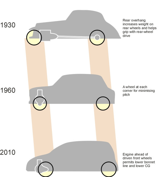
Most cars nowadays have four wheels, and we rarely question whether in fact this is the right number. Still less do we question how the wheels should be arranged. It just seems natural to put two at the front and two at the back, with a greater or lesser degree of overhang at either end. For many years, it was fashionable to have a long tail, which reflected early ideas about streamlining. But during the 1960s, aiming to minimise the pitching motions that have always bedevilled small saloons, BMC designer Alec Issigonis placed the rear wheels further aft than was usual at the time [22]. This arrangement also freed space within the passenger compartment. Issigonis’ cars were roomy and rode well, but the wheel layout resulted in a characteristic four-square appearance that not everyone liked. Eventually, other designers followed suit, but they have since tended to mount the engine slightly ahead of the front axle, which leads to a more pronounced front overhang instead.
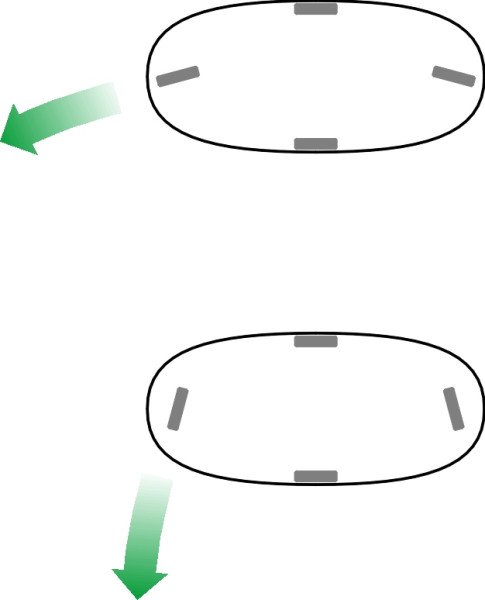
From time to time, designers have tried a more radical approach, with the wheels arranged in a diamond formation as shown in figure 3. In some cases the diamond layout is really a two-wheeled motorcycle with small wheels as outriders that keep the machine upright when standing still. But many are proper four-wheeled cars. Details of several examples can be found in a book by Stephen Vokins [17]. One of the most rational was the Ellipsis, exhibited at the 1992 Paris Motor Show and the creation of industrial designer Philippe Charbonneaux. Note that for a vehicle of this kind, both the front and the rear wheel must swivel when the car steers round a curve, and depending on the amount of lock available, this layout makes the car more manoeuvrable than a conventional 4-wheel model. Figure 4 shows that if the range of steering angles were \(\pm 90^{\circ}\), it could in theory turn within its own length.
Figure 3
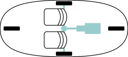
Figure 4
Three wheels
For a small vehicle, the three-wheel layout seems a logical choice, with less weight, less to go wrong, and less expense. At various times during the last century, the three-wheeler provided a real alternative. Examples include the lightweight sports cars produced by the Morgan company in Britain. Powered by a chain drive to the single rear wheel, they were raced successfully during the 1930s, and some still survive. After 1945, several German and Italian companies, exploiting lightweight construction skills honed in the wartime aircraft industry, developed a range of three-wheel ‘bubble cars’ that were totally enclosed and could be used as family runabouts.
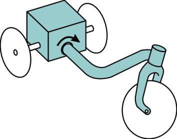
Most three-wheel cars have two wheels at the front and a single wheel at the rear, because as we shall see later, this arrangement is more stable than having the single wheel in front. On the other hand, the single front wheel has a significant advantage, because the steering linkage is simpler and lighter than the Ackermann assembly needed for a conventional front axle (see Section C0504). One solution is to keep the single front wheel but make the vehicle lean from side to side (there are several ways to do this, one of which is to articulate the chassis so the front leans while the rear stays upright as shown diagrammatically in figure 5). A leaning machine can corner like a motorcycle at a respectable speed without overturning, and the track width can actually be reduced to create a very light and compact vehicle in which the passenger sits behind the driver. Since 1980, at least four designs have emerged along these lines, although as far as the author is aware, none are currently in production. Further details are set out in Table 1.
Figure 5
| Model | Year | Details | Source |
| Lean Machine | 1982 | Single-seat commuter runabout with handlebar controls, capable of 60 mph. Two prototypes were built by General Motors. | [4] [9] |
| F300 Life-Jet | 1997 | Concept car by Mercedes-Benz: it could lean up to 30\(^\circ\); unlike the other three models in this table, the single wheel was at the rear. | [5] |
| Carver | 1997 | A design originating in Holland; the prototype was capable of 115 mph. | [19] [23] |
| CLEVER | 2006 | £1.5m collaborative project between the Technical University of Berlin and BMW, the Compact Low Emission VEhicle for uRban transport has a hydraulic tilting mechanism; the rear 2 wheels and engine stay upright. The 230 cc engine is fuelled by Liquid Natural Gas. | [16] |
Two-wheelers
Since we’ve got down to three wheels, we might as well keep going: what about two? To most people, a two-wheeled vehicle is by definition a motorcycle, which cannot easily be enclosed to protect the rider from the weather, and it won’t stand up by itself. Yet in 1912 the Russian aristocrat Count Peter Schilovski contrived a 2.7 ton petrol-engined two-wheeler that could seat five passengers [2] [18]. It was stabilised by bleeding off 10% of the engine power to drive a 100 cm diameter gyroscope at between 2000 and 3000 rpm. The Schilovski Gyrocar was built in Birmingham by Wolseley. It worked, but did not go into production.
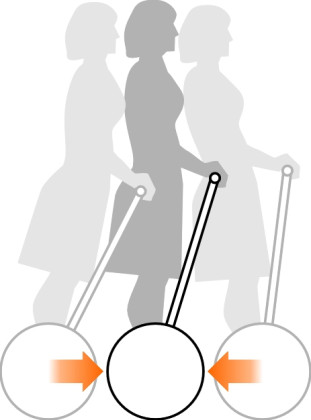
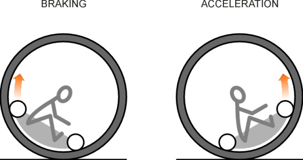
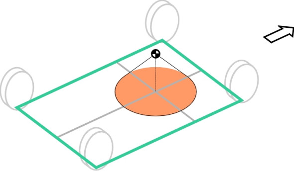
A vehicle that did go into production was the Segway, the conception of engineer and entrepreneur Dean Kamen. You can still buy one. Unlike those on a motorcycle, the wheels, which are powered by two separate electric battery motors, are arranged side-by-side, and the rider stands on a platform between them. The vehicle balances itself in the same way that a sea lion balances a beach ball on its nose, by rapidly adjusting its position back and forth to counter any small deviation from equilibrium (figure 6); these movements are controlled automatically by gyroscopes. To make it follow a curved path, the electric motors must drive the wheels at different speeds. Turns are controlled by means of a tiller that the rider moves left or right. This remarkable design is based on experience that Dean Kamen acquired over years of developing mobility aids for the disabled, and the development programme was supported by some of the largest investment organisations in the USA. The story of its inception has been recorded in detail by Stephen Kemper [13].
Figure 6
Mono-wheels
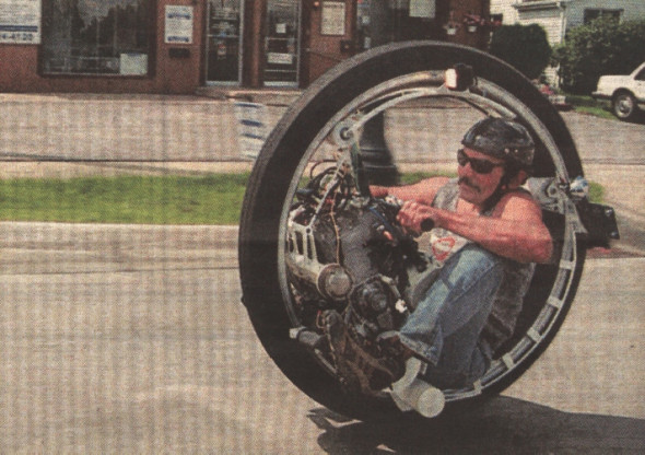
If two wheels, why not one? The unicycle was once a popular attraction in stage and circus shows. Perched on a saddle with nothing else to hold on to, the rider stayed upright by pumping the pedals backwards and forwards. But a single-wheeled vehicle is easier to ride if your body weight is concentrated below axle level so you hang like a pendulum inside the rim, and you might be surprised at how many inventors have built machines along these lines [26]. The earliest examples appeared during the 19th century, a series of pedal-driven monocycles stimulated perhaps by the ‘penny-farthing’ bicycle [6], and the idea never really went away. Power-driven machines followed, ranging from Mr Purves’ gasoline-engined Dynasphere of 1930 [20], to Kerry McLean’s Mini Monowheel of the present day (see figure 7). The Mini Monowheel holds the current world speed record of 86.5 km/h [1].
Figure 7
A monowheel has no suspension springs, and although its large wheel diameter helps to smooth out the bumps, there is a major drawback: control. It is not easy to make a sharp turn, and the passenger compartment tends to oscillate like a pendulum whenever engine torque is applied (figure 8). If you were to lock the brakes, you would go round and round with the rim.
Figure 8
A question of stability
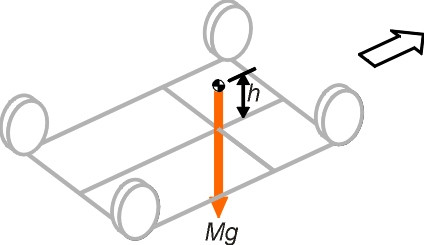
It seems a vehicle can be built around almost any wheel configuration that one cares to imagine. Yet the large majority all cars on the road today have four wheels arranged at the corners of a rectangle. This arrangement confers a degree of stability that cannot easily be bettered with any other configuration, regardless of the number of wheels. To see why, we must view the vehicle in three dimensions and consider the forces acting on it. As a starting point, figure 9 shows the four wheels and the centre of mass, which lies at a distance \(h\) above the road surface, slightly ahead of the midpoint.
Figure 9
The stability cone
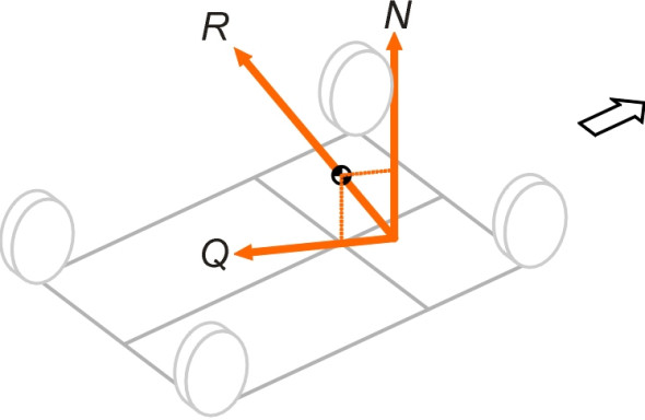
Only three types of force can act externally on the car that is travelling along a smooth horizontal surface: (a) the vertical reactions from the road that press upward on the tyres, (b) the friction forces between the tyres and road, and (c) aerodynamic forces. Here we shall ignore the aerodynamic forces, although they can affect stability in a strong wind. The vertical reactions can all be replaced by a single vertical reaction \(N\). If the mass of the vehicle is M, this reaction must be equal to \(Mg\). Similarly, the friction acting on the tyres can be resolved into a single shear force \(Q\). We now have only two forces acting on the car, as shown in figure 10. Assuming that any disturbance arising from rotational inertia is small enough to be ignored, if we now take moments about any axis passing through the centre of mass, equilibrium requires that the net couple exerted by these two forces must be zero. It follows that \(N\)and \(Q\) lie in the same vertical plane, and their resultant \(R\) passes through the centre of mass (figure 11).
Figure 10
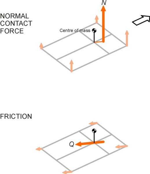
Figure 11
Now let’s see what happens when the driver attempts some manoeuvres. When the vehicle is moving in a straight line at constant speed, the vertical reaction is located directly under the centre of mass. \(Q\) is zero. (In fact, neither of these statements is quite true because tractive forces are needed to maintain speed against several forms of resistance, but we’ll ignore them and assume that stability is only called into question when the driver brakes, accelerates, or steers round a curve.)
If the driver applies the brakes, then a non-zero retarding force \(Q\)will oppose the vehicle’s motion. Under acceleration, \(Q\) will switch to the opposite direction, pushing the vehicle forward. To keep things simple, we’ll suppose the driver brakes or accelerates at a constant rate so that \(Q\) is constant. Alternatively, the driver could maintain a constant speed but steer round a curve of fixed radius. In this case, \(Q\) must act laterally. Or we might have some combination of (a) a steady longitudinal braking or acceleration force and (b) a steady lateral cornering force.
Whenever \(Q\) changes from zero to some finite value, there must be a compensating shift in the location of the vertical reaction \(N\). Otherwise, the resultant of \(N\) and \(Q\) would no longer pass through the centre of mass. It is this shift that engineers refer to as load transfer (see Section C2009). For example, under braking \(N\) will shift forward, directly ahead of the centre of mass. Under acceleration it will shift rearward. When cornering, it will shift towards the outside of the curve. In figure 10, we show a vehicle that is turning to the left and braking simultaneously, so \(N\) is shifted forward and to the right. More generally, we need to know how far it might move as a result of any conceivable manoeuvre, in other words, if we denote the shift by \(s\), what is the largest value of \(s\) we are likely to encounter, and in what direction?
At this point we make two more simplifying assumptions. First, we assume that the maximum friction force equals the vehicle weight times the coefficient of friction so that
(2)
\[\begin{equation} Q_{\max} \quad = \quad \mu Mg \end{equation}\]This is not quite true because the relationship between friction and normal contact force for rubber tyres is not linear (see Section C1717), but it won’t greatly affect the outcome. Secondly, we assume that the coefficient of friction is the same in all directions: this is tantamount to saying that the ellipse of friction for the tyres is in fact a circle.
Figure 12
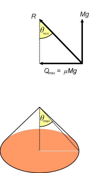
If we now look at the vertical plane that passes through the centre of mass and the vertical reaction (figure 12), we see that the largest possible angle \(\theta_{\max}\) between the overall resultant \(R\) and the vertical is governed by the ratio of \(Q_{\max}\) to \(N\); specifically
(3)
\[\begin{equation} \tan {\theta_{\max }} \quad = \quad \frac{Q_{\max}}{N} \quad = \quad \frac{\mu Mg}{Mg} \quad = \quad \mu \end{equation}\]Therefore the vertical reaction can lie anywhere within the base of a cone whose vertex is located at the centre of mass, and whose base, which lies on the road surface, subtends at the vertex an angle equal to \(\textrm{arctan} \mu\)(figure 12). If the height of the centre of mass above the road surface is \(h\), the radius of the base determines the maximum shift \(s_{\max}\), and this radius is given by
(4)
\[\begin{equation} s_{\max} \quad = \quad h \tan{\theta_{\max }} \quad = \quad h \mu \end{equation}\]We can represent the base as a disc painted on the ground with its centre directly below the centre of mass (it is coloured orange in figure 12). Now let’s move the vehicle out of the way, and hammer a pin into the ground at the centre of each tyre contact patch. Then we mark out the envelope of the contact patch centres by looping a piece of string round the pins and drawing it tight. The string is shown coloured green in figure 13.
Figure 13
A little thought should convince you that the car cannot overturn if the stability cone lies within the envelope. But if the cone overlaps the boundary, it is possible for \(N\) to move outside. Such an event would imply negative contact forces at one or more wheels on the opposite side of the car, in other words, the wheels would have to be glued to the road to prevent them from lifting off the road. It is a widely recognised requirement in car design that the tyres should reach the limit of their grip before this can happen. In other words, the car skids before it overturns [7]. Hence we need the stability cone to lie entirely within the contact patch envelope; if not, it is theoretically possible for the driver to execute a manoeuvre that turns the car over. This is one reason why designers keep the centre of mass as low as possible, because any reduction in \(h\) immediately reduces the radius of the cone.
Now let us try to fit the stability cone within some alternative wheel plans. Some options are shown in figure 14. The rectangle at the top represents a conventional car with a wheel at each of its four corners. Below is a diamond layout with a single wheel in front, a single wheel behind, and two wheels arranged amidships. At the bottom is the more familiar three-wheeler, with a single wheel at the front. One can see that the rectangular envelope encloses a larger disc than a diamond envelope of the same overall width. In other words, the car with the rectangular layout can survive greater friction forces without overturning. So we can rule out the diamond layout. Note also that the rectangular layout cannot be improved by increasing the number of wheels to six or eight, say. Assuming that the overall width is constrained by width of a typical parking space, adding more wheels doesn’t change the envelope.
Figure 14
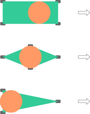
Figure 15
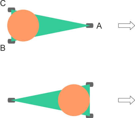
What about the three-wheeler? At first sight it appears that a three-wheeler is no better than a diamond. However, it can be made reasonably safe provided the single wheel isn’t at the front. As shown in figure 15, a single wheel at the front allows the car to overturn about either side AB or AC of the contact envelope as the load transfers forwards and sideways under a combination of braking and cornering. But if it is at the rear, the necessary load transfer can only be achieved by a combination of traction and cornering forces: the acceleration must be so powerful that the car tips over backwards and to one side. In practice, few three-wheelers have sufficient engine power to do this.
Will your car roll over?
As you would expect, the saloon car today is designed with its centre of mass as close as possible to the road surface, typically at a height of between 0.5 and 0.7 m [8] [10]. Consequently, it would take a high level of centripetal acceleration, say 1.1 to 1.5 \(g\), to roll a car under any combination of steady cornering and braking forces. This in turn would require an unusually high coefficient of friction between the tyres and the road. With their higher centre of mass, SUVs and light goods vehicles are less stable, while heavy trucks are distinctly vulnerable, partly because the centre of mass of the payload may lie a considerable distance above the road surface. A truck may therefore overturn when subject to a comparatively modest cornering force of 0.25 \(g\) [11].
However, the risks are actually greater than these figures would suggest, mainly for two reasons. The first has to do with body ‘roll’. No vehicle stays perfectly upright when travelling round a curve. The body tilts outwards so the centre of mass moves away from the central axis of the car, carrying the stability cone with it. This in turn may carry the resultant normal contact force outside the contact patch envelope, which is one of the reasons why designers configure the suspension so as to control the degree of body roll within prescribed limits (you’ll find more on the question of body roll, which affects not only stability but vehicle handling in a broader sense, in section C0414). Secondly, our model breaks down during a transient manoeuvre. For example, during a sudden lane change a heavy truck may oscillate first to one side and then the other, which can tip the vehicle over at a relatively low \(g\)-force. So strictly speaking, the answer to the question ‘will your vehicle roll over?’ is yes. But the question is not a helpful one. Any vehicle can be made to roll under extreme or freakish circumstances, and what the motorist really wants to know is ‘what sort of vehicle is least likely to roll over?’ You will be pretty safe in a modern family saloon car, but less so in other configurations. In particular, the risk increases with height, so SUVs and MPVs will roll over in circumstances where an ordinary car would not.
Conclusion
Of all the possible layouts for a family car, it seems that the conventional four-wheel layout with a wheel close to each corner provides the maximum stability, and for this reason alone it will probably remain the standard pattern for a while. Not only does it provide the most stable platform, but it also keeps the wheels, suspension and drive shafts clear of the passenger compartment. Historically, however, as vehicle technology has evolved over time, the axle positions have moved backwards and forwards relative to the body envelope. During the 1920s and 30s, it made sense to have the front wheels ahead of the engine, and it was fashionable to have a long tail at the rear (figure 16). During the 1950s, some manufacturers abandoned the rear overhang in favour of a wheel at each corner. Nowadays, the rear wheels have moved even closer to the tail, but the engine has shifted forward, creating a considerable overhang at the front. In this sense, the modern motor vehicle is set up very much like the cars of yesteryear, but in reverse.
Figure 16
Appendix: Taking the average
Figure 17
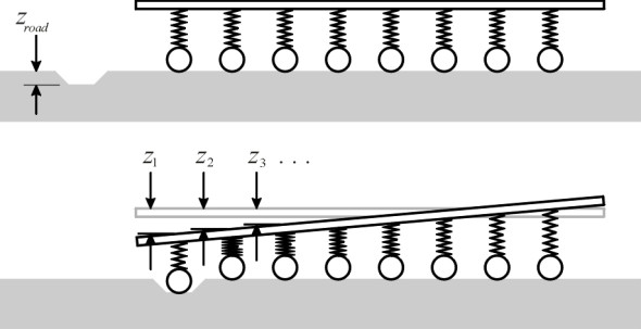
Let’s imagine a vehicle with \(n\) equally spaced axles as shown in figure 17. For the moment, we’ll assume that the vehicle has three axles or more, so \(n\) > 2. The front axle is displaced downwards as the wheels fall into a shallow trough of depth \(z_{road}\) and we want to determine the displacement at the midpoint of the chassis. To do this, we must take into account the fact that each set of springs is compressed by a different amount, and in fact the springs towards the rear will stretch a little. Starting at the front, we’ll number the axles \(i\) = 1, 2, 3, .., \(n\), and denote by \(z_{i}\) the displacement of the chassis at axle \(i\). Given the displacement \(z_{1}\) at the leading axle and the displacement \(z_{n}\) at the trailing axle, we can work out the displacement at each of the intermediate axles from simple geometry because successive values change by equal steps between \(z_{1}\) and \(z_{n}\). The required expression turns out to be
(5)
\[\begin{multline} z_{i} \quad = \quad \left( \frac{n \; - \; i}{n \; - \; 1} \right) z_{1} \;\; + \;\; \left( \frac{i \; - \; 1}{n \; - \; 1} \right) z_{n}\\ (n = 3, 4, 5, \ldots ; \; i = 1, 2, \ldots{} , n) \end{multline}\]We now want to work out an expression for the increase in the load carried by each axle when the front axle encounters the trough. Call the increase in load for the \(i^{th}\) axle \(P_{i}\). If the springs are linear, the increase in load divided by the increase in spring deflection is equal to a constant \(k\) which we call the spring stiffness (here we are taking compressive deflection as positive, so an increase in deflection means that the spring is squashed relative to its initial state). For the first axle, where the increase in deflection is \(z_{1}\) – zroad, we have
(6)
\[\begin{equation} P_{1} \quad = \quad k(z_{1} \; - \; z_{road}) \end{equation}\]It has a negative value, indicating that the spring is actually stretched a little and the load is reduced. For the second and remaining springs, the increase in deflection is just \(z_{i}\), so we have
(7)
\[\begin{equation} P_{i} \quad = \quad kz_{i} \end{equation}\]which, if we substitute for \(z_{i}\) via equation 5 becomes
(8)
\[\begin{multline} P_{i} \quad = \quad \frac{k}{(n - 1)} z_{i} \left[ (n - i)z_{1} \;\; + \;\; (i - 1) z_{n} \right] \\ (n \ge 3 ; \quad i \; = 1, 2, \ldots , n) \end{multline}\]We can now sum the individual changes in axle load thus:
(9)
\[\begin{multline} \sum \limits_{i \; = \; 1}^n {P_i} \quad = \quad k(z_{1} \; - \; z_{road}) \;\; + \;\; \sum \limits_{i \; = \; 2}^n {\frac{k}{(n - 1)} z_{i} \left[ {(n - i)z_{1} \;\; + \;\; (i - 1)z_{n}} \right]} \\ (n \;\; \ge 3) \end{multline}\]But since the total load on the axles hasn’t changed, this sum must be zero. If we evaluate the summation in the usual way and then equate the right hand side of equation 9 to zero, after some simplification we arrive at the result
(10)
\[\begin{equation} z_{road} \quad = \quad \frac{n}{2} \left(z_{1} \; + \; z_{n} \right) \end{equation}\]Notice that on the right-hand side of equation 10 the term \((z_{1} + z_{n})/2\) is identical with the displacement at the chassis midpoint – precisely the value we are seeking. It follows that the midpoint displacement is equal to the leading axle displacement \(z_{road}\) divided by \(n\), so that the ratio \(\rho\) of midpoint chassis displacement to leading axle displacement is given by
(11)
\[\begin{multline} \rho \quad = \quad \frac{1}{n} \\ (n \ge 3) \end{multline}\]The formula also happens to work for a vehicle with a single axle and for a vehicle with two axles (\(n\) = 1 and \(n\) = 2) as can easily be demonstrated by working out these two cases separately.
This is such a simple result that you might guess there’s an easier way to derive it, and there is. It makes use of a principle first proposed by the physicist James Clerk Maxwell in 1864, which is still used by civil engineers to predict the displacements occurring within a rigid structure. By ‘rigid’ we mean something like a railway bridge that is firmly anchored to the ground but whose parts will distort slightly under the action of their own weight together with that of each passing train. The displacements everywhere must be linearly proportional to the load involved. The Theorem of Reciprocal Displacements expresses a kind of symmetry between the displacement at two different points: if you apply a load at A and measure the displacement at B, you will get the same answer as if you applied the load at B and measured the displacement at A (the displacement at A must be measured in the same direction as the original load at A, and similarly, the load at B must be applied in the same direction as the displacement originally measured at B; for a more complete explanation see for example [14]).
The theorem seems like a conjuring trick, but it works, and it greatly simplifies the multi-axle vehicle problem. Suppose first that we apply a load \(P\) vertically downwards to the midpoint of the chassis. This load will be shared equally among all the axles. The suspension at any axle \(i\) will therefore carry a load \(P/n\). If the stiffness of each spring is \(k\), the increase in deflection \(\delta_{i}\) must be equal to the applied load divided by stiffness, so that
(12)
\[\begin{multline} \delta_i \quad = \quad \frac{P}{nk} \\ (n \ge 3; \quad i = 1, 2, \dots , n) \end{multline}\]Now let’s look at the leading axle. If we apply a load \(P\) vertically downward to the chassis at the position of the leading axle, Maxwell’s theorem says that the displacement of the chassis midpoint will be the same as the displacement previously observed at the leading axle when the load was applied to the midpoint, i.e, \(P/nk\) vertically downwards. But what we really want to know is the displacement \(\delta\) at the centre when the leading wheels roll into a trough of depth \(z_{road}\). This encounter is equivalent to decreasing the compression force within the leading spring by an amount \(kz_{road}\). In other words, we have effectively superimposed a downward load on the chassis equal to \(kz_{road}\) at the leading axle. We therefore substitute \(kz_{road}\) for \(P\) in equation 12 and cancel the factor \(k\) from the top and bottom to get the value on the right-hand side as \(z_{road}/n\). In other words
(13)
\[\begin{multline} \delta \quad = \quad \frac{z_{road}}{n} \\ (n \ge 3 ; \quad i = 1, 2, \dots , n) \end{multline}\]This result doesn’t just apply to encounters involving the leading axle. When the second axle reaches the trough, exactly the same reasoning applies, and so on for every axle. Hence the effect of a bump on any axle is attenuated at the midpoint of the vehicle by a factor of \(1/n\). But there is a catch. With \(n\) axles, although the displacement sensed by the driver is reduced by a factor of \(n\), the bump is transmitted to the driver \(n\) times!
Loose ends
equation 1 gives a simple formula for the ‘gain’ \(\rho\) for the response at the vehicle midpoint when any one of the axles is displaced over a bump or depression in the road surface. But the occupants of a vehicle don’t always sit in the middle of the chassis. What can we say about the displacements elsewhere? Would the occupants be better off sitting, for example, at the rear?
Acknowledgements
Picture on opening page: Camper van by Penny Wright
Figure 7: Photo kindly provided by Kerry McLean
Revised 16 February 2015