C.0418
Oversteer and understeer
For about 40 years, manufacturers have been selling cars that are safe to drive. A safe car is predictable, so that if called on to make a sudden swerve, the driver knows roughly what the car will do. Cars haven’t always been like this. Around 1900, on a wet road many would spin round unexpectedly and face the wrong way, a disconcerting trait that drivers found difficult to manage. There were two main causes. The first was loss of grip at the rear: early cars had brakes on the rear axle only, and any car will spin if the rear wheels lock while the front wheels continue to rotate (Section C0415). The cure was simply to install brakes on all four wheels and to proportion the braking effort in a measured fashion between them. The second cause was more mysterious, and like the 3-dimensional ‘spin’ to which aircraft were prone (and still are), it took many years to tame. It was a characteristic essentially built into the suspension design: oversteer. Of all the handling quirks that engineers confronted during the last century, oversteer was for a time the most challenging and the least well understood.
What is ‘oversteer’?
The terms ‘oversteer’ and ‘understeer’ first appeared in an unpublished GM report of 1937 by Maurice Olley [4], originally a Rolls Royce engineer who had emigrated to GM to work on the Cadillac [12]. In the USA today, understeering behaviour is sometimes known as ‘pushing’ or ‘ploughing’, while a car that oversteers is said to have ‘loose’ steering. To understand what is going on, we need the thin car model that was described earlier in Section C0415. The model is convenient because it has only one front wheel. The angle of this wheel to the longitudinal axis at any given moment is called the steering angle. It reflects what the driver is trying to do by manipulating the handwheel (we will use ‘handwheel’ instead of the more familiar term ‘steering wheel’, which can cause confusion).
Neutral steer
Figure 1
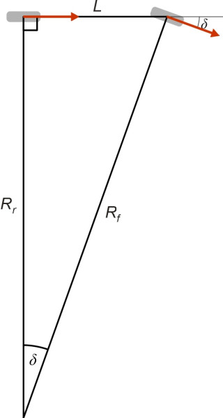
Suppose the driver holds the handwheel in a steady position while the car is travelling at constant speed \(V\). The steering angle – the angle of the front wheel to the car body - will remain fixed at a certain value \(\delta\) say. If its wheels behaved like blades and travelled exactly where they were pointing without any tyre slip, the thin car would trace out a circular path. The rear wheel would follow a circle of radius \(R_r\) and the front wheel a circle of radius \(R_f\). From figure 1 we see that \(L \, = \, R_{r} \tan \delta\), and if \(\delta\) is small, which it usually is, we can take the radius of the curve travelled by the front wheel and the rear wheel as the same, and call it simply \(R\). Hence for the whole vehicle:
(1)
\[\begin{equation} L \quad = \quad R \tan \delta \end{equation}\]Conversely, if we start with a curve of radius \(R\) fixed in advance, at what angle must the front wheel be steered to carry the car round that curve? Re-arranging equation 1, and noting that for small steering angles, the tangent of an angle is approximately equal to the value of the angle expressed in radians, we get
(2)
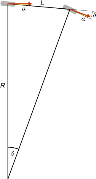
\[\begin{equation} \delta \quad \approx \quad \frac{L}{R} \end{equation}\]Of course, pneumatic tyres don’t roll in exactly the direction they are pointing (Section C1717). So let’s suppose that the front wheel slips at a small angle \(\alpha\) to its axis, and the rear wheel similarly. If the two slip angles are identical, effectively, the whole vehicle including both wheels will be angled bodily relative to its path along the road: it drifts at an angle \(\alpha\) relative to its previous heading. But its path is unchanged, and therefore it will continue to follow a curve whose radius \(R\) remains unaltered (figure 2). Now, equation 1 and equation 2 only hold for a car with equal slip angles front and rear. For such a car, the steering angle required to maintain a curve of any given radius is called the Ackermann angle, and its value is independent of speed. The driver applies exactly the same steering action at 10 km/h as she does at 100 km/h. This behaviour is referred to as neutral steer, and it defines the boundary between understeer and oversteer.
Figure 2
Understeer and oversteer
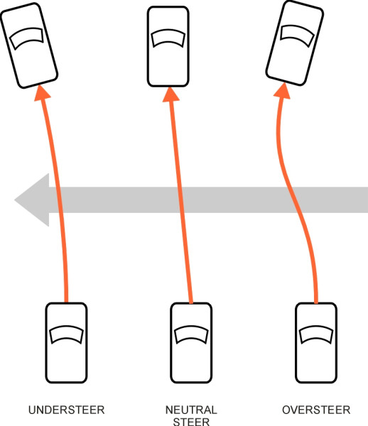
On a real car, the front and rear slip angles are rarely equal and its behaviour must lie on one or other side of the boundary. If the steering angle is greater than the Ackermann angle, the vehicle is said to understeer. In non-technical terms, the steering has to work hard, with the front wheel swivelling further than would be necessary in the neutral case. On the other hand, if the steering angle is less than the Ackermann angle, the car is said to oversteer [1] [7]. The car will turn with relatively little movement of the front wheels. This distinction is more important than might it might at first appear, and to see why, we must find a mathematical expression for the relationship between \(L\), \(R\), \(V\), and \(\delta\) that takes the slip angles into account. Although the behaviour of a car in three dimensions on real roads is complicated, the main features can be understood quite easily with the aid of the thin car model.
Figure 3
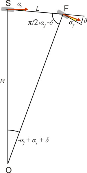
The cornering equation
The aim now is to determine the relationship between steering angle and curve radius when the front and rear slip angles \(\alpha_f\) and \(\alpha_r\) are no longer equal. We’ll follow the argument previously set out by vehicle handling specialists (see, for example, [6]), except that we shall express the angles in radians, not degrees. The new geometry is shown in figure 3. As before, the front and rear wheels follow slightly different radii. We take the rear wheel as our datum, and designate the radius \(R\). Applying the sine rule to triangle OSF shows that
(3)
\[\begin{equation} \frac{L}{\sin \left( \delta - \alpha_f + \alpha_r \right)} \quad = \quad \frac{R}{\sin \left( {\frac{\pi}{2} - \delta + \alpha_f} \right)} \end{equation}\]After some rearrangement together with some fairly cavalier approximations we end up with
(4)
\[\begin{equation} \delta \quad \approx \quad \frac{L}{R} \; + \; \alpha_f \; - \; \alpha_r \end{equation}\]Since we have already decided that the car is travelling at speed \(V\), we can work out the side forces on the tyres, deduce the values of the two slip angles, and substitute them in equation 4 to achieve our goal. The side forces are not identical, if only because the weight of the car is not shared equally between the front and rear axles. Usually, the greater proportion will be carried by the front axle and the remainder by the rear axle. Let the load on the front axle be \(P_f\) and the load on the rear axle \(P_r\). Each axle has to provide a side force equal to the axle load times the speed squared divided by \(R\). Hence
(5)
\[\begin{equation} \text{Front side force} \quad = \quad Q_{f} \quad = \quad \frac{P_{f}V^2}{R} \end{equation}\](6)
\[\begin{equation} \text{Rear side force} \quad = \quad Q_{r} \quad = \quad \frac{P_{r}V^2}{R} \end{equation}\]What slip angles will be needed to develop these forces? From equation 1 in Section C1717 we know that for any tyre, the slip angle equals the side force divided by cornering stiffness. If we denote the front and rear cornering stiffness per axle respectively by \(k_{Cf}\) and \(k_{Cr}\), then
(7)
\[\begin{equation} \alpha_f \quad = \quad \frac{Q_{f}}{k_{Cf}} \quad = \quad \frac {P_{f} V^2}{k_{Cf} R} \end{equation}\](8)
\[\begin{equation} \alpha_r \quad = \quad \frac{Q_{r}}{k_{Cr}} \quad = \quad \frac {P_{r} V^2}{k_{Cr} R} \end{equation}\]Substituting these expressions into equation 4 yields
(9)
\[\begin{equation} \delta \quad \approx \quad \frac{L}{R} \; \; + \; \; \left( \frac {P_f}{k_{Cf}} \; - \; \frac{P_r}{k_{Cr}} \right) \frac{V^2}{R} \end{equation}\]Notice that the expression \(V^{2}/R\) on the right hand side is by definition equal to the lateral acceleration imposed on the vehicle. The expression inside braces is usually abbreviated to the symbol \(K\). It is known as the understeer gradient because if we plot the curve of \(\delta\) against lateral acceleration, the graph will be a straight line with \(K\) as the slope. And if \(K\) is negative, the car understeers, while if it is positive the car oversteers. Note that the units of \(K\) here are radians m\(^{-1}\) s2 as opposed to the more usual degrees m\(^{-1}\) s2.
So now we have the final version of the cornering equation thus:
(10)
\[\begin{equation} \delta \quad \approx \quad \frac{L}{R} \;\; + \;\; K \frac{V^2}{R} \end{equation}\]The cornering equation tells us straight away what steering angle is needed to traverse a given curve at a given speed, and also shows how the steering angle must change as the speed of the car increases. Some plots of \(\delta\) as a function of \(V\) for a car of wheelbase 2.5 m travelling on a curve of radius 500 m are laid out in figure 4. Each line corresponds to a different suspension set-up. The horizontal line in the middle represents the ‘neutral steer’ case where the slip angles front and rear are equal. To execute the 500 m curve, the required steering angle for this particular car is around 0.005 radians or \(0.3^\circ{}\) regardless of speed.
Figure 4
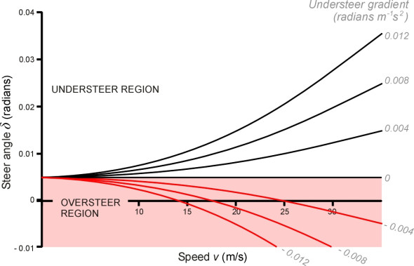
Above the neutral steer line is the understeer region. Each black line corresponds to a different suspension set-up as measured by the value of its understeer gradient \(K\) in equation 10. Each line slopes up to the right, indicating (as one might expect) that as the speed increases the driver must apply more steering angle to hold the vehicle on the 500 m curve. Furthermore, as the degree of understeer increases, we move upwards from one curve to the next, showing that increasing levels of understeer require increasing amounts of steering angle. A car that understeers can be hard work for the driver. It resists turning, as though it would prefer to carry straight on.
Below the neutral steer line is the oversteer region. Each line slopes down to the right, meaning that if the driver decides for some reason to speed up while travelling on a circular bend, she must reduce the steering angle, which is perhaps the opposite of what one might expect. Oversteer is associated with sports cars. It makes the handling feel more responsive so the drivers can ‘flick’ the car into a curve with relatively little effort.
Instability
An oversteering car may sound like a good idea except that for a given handwheel angle, the path radius will decrease with increasing speed. In other words, if you step on the accelerator pedal the car will veer towards the insideof the curve – again the opposite of what you might expect. With an understeering vehicle the response is more natural: an increase in speed tends to carry the vehicle off the outside of the bend [13]. Furthermore, a negative understeer gradient in equation 10 implies that at high speeds, the steer angle that is needed to hold the car on a given curve radius is negative. To follow a curve whose radius falls in value at some point after entry, the driver must steer towards the centre of the curve and then apply an immediate correction in the opposite direction to hold the vehicle on course.
The undriveable car
But the driver may never reach that stage, because there is an intermediate speed at which any change in steering angle leads to infinite yaw rate: the car is fundamentally unstable. The critical speed \(V_{crit}\) occurs when the graph crosses the horizontal axis in figure 4. At that speed, in equation 10 we have \(L \; + \; KV^{2} = 0\), which leads to
(11)
\[\begin{equation} V_{crit} \quad = \quad \sqrt {\frac{- L}{K}} \end{equation}\]For example, if we set up the car with an understeer gradient \(K \; = \; -0.004\) rad m\(^{-1}\) s2, we see that the graph crosses the horizontal axis when the speed is about 25 metres per second. To see what happens when the car approaches this speed, it helps to re-arrange equation 10 in the form
(12)
\[\begin{equation} R \quad = \quad \frac{ \left( L \; + \; KV^2 \right)}{\delta} \end{equation}\]We’ll imagine the driver carrying out a test on a circular track of radius 500 m. Initially, the vehicle is moving slowly, and the numerator on the right-hand side of equation 12 is positive. As the driver accelerates, since \(K\)is negative, the path radius will tend to fall as \(V\) increases. The driver must keep to the 500 m radius, so she reduces the steer angle \(\delta\) accordingly. When \(V\) is almost equal to 25 metres per second, both numerator and denominator become very small, and the slightest change in steer angle will cause the vehicle to alter course dramatically. At the critical point itself when \(L \; + \; KV^{2} = 0\), the curve radius is undetermined, and the driver is caught up in a mathematical singularity. Any steering action results in a spin. To put it another way, at the critical speed, the steer angle required to hold a curve of any radius is zero [16].
Stability against lateral forces
A car may have to resist lateral forces even when travelling in a straight line, forces that tend to push it to one side. In principle, such a force could act anywhere along the car body, but one location has special significance. We define the Neutral Steer Point (NSP) as the point at which a lateral force will shift the car bodily sideways without inducing any yaw [14] so that the car ‘crabs’ to one side without actually changing its orientation. It turns out that the NSP for an understeering car lies behind the centre of mass, while that for an oversteering car lies ahead of the centre of mass. In fact, the position of the NSP relative to the centre of mass provides an alternative criterion for oversteer, and is the one originally developed by Maurice Olley: the slip angle criterion and Olley’s criterion are mathematically equivalent. Since manufacturers aim for a modest amount of understeer for all normal driving conditions, they plan the layout of each new model so that the NSP trails the CoM by a safe margin, typically between 0.05 and 0.07 of the wheelbase [8].
One kind of lateral force commonly encountered during everyday driving conditions is the force produced by a lateral slope or crossfall in the road surface. On a lateral slope, a component of the car’s weight acts at right angles to the direction of motion, which causes each of the four tyres to deviate slightly at an angle to the direction in which it is pointing. This angle is just the slip angle mentioned earlier. But the slip angle at the front is not necessarily the same as the slip angle at the rear. Since the resultant lateral force passes through the centre of mass, an understeering car with its more ‘compliant’ axle at the front tends to yaw down the slope as shown in the diagram on the left-hand side of figure 5. In other words, it points more-or-less in the direction in which it deviates from the driver’s intended course. The driver will need to keep the handwheel off-centre to maintain position in the middle of the traffic lane, but the corrective action is obvious and the system is inherently stable. An oversteering car, on the other hand, will be difficult to handle. While the car crabs bodily down the slope as before, there is more resistance at the front axle so the car yaws in the opposite direction as shown in the diagram on the right-hand side of figure 5. It deviates in one direction but it points in the other. Which way should the driver turn the handwheel, and when?
Figure 5
Another kind of lateral force arises from cross-winds, which sometimes cause trouble on exposed sections of road, especially on high bridges. It is less easy to predict the effect of a cross-wind because the aerodynamic force doesn’t usually pass through the centre of mass, nor does it pass through the NSP. The point on the car body at which the crosswind acts is known as the centre of pressure, and as described in Section C1416, it usually lies ahead of the NSP, so that the vehicle turns away from the wind.
Factors affecting oversteer
Since oversteer is caused by a relative shortfall in cornering stiffness of the rear tyres, the construction of the tyres is important; the front and rear pairs should be appropriately matched. But what counts as a ‘shortfall’ depends partly on the loading applied to each of the four wheels, which in turn depends on the weight distribution between front and rear axles together with the suspension characteristics, as summarised in table 1.
| Steering | Factor |
| OVERSTEER | Rearward weight distribution resulting from (for example) a rear engine [5] |
| Soft front springs and stiff rear springs, which make the rear suspension stiffer in roll than the front suspension resulting in increased lateral load transfer, see [15] also Section C2009 | |
| UNDERSTEER | Forward weight distribution, see [5] |
| Stiff front springs and soft rear springs, which make the front suspension stiffer in roll than the rear suspension, see [15] | |
| Anti-roll bars front |
However, the degree of oversteer or understeer is not fixed for any given vehicle, because the front and rear tyre slip angles can vary from moment to moment, influenced by acceleration and braking which use up a significant proportion of the total grip [10]. They way they do this depends on whether the vehicle is front-wheel drive, rear-wheel drive, or 4-wheel drive. For example, the cornering stiffness of the rear wheels on a rear-wheel drive car is to some extent compromised when the driver applies power, because by applying traction in the fore-and-aft direction, the rear wheels use up some of the friction, which effectively raises the slip angle. Hence a rear-wheel drive car tends to oversteer on the exit from a bend [11]where heavy throttle can make the car spin. The opposite is true of a front wheel drive car, which tends to understeer, and when accelerated hard tends to carry straight on. Oversteer is also affected by small changes in the alignment of the wheels as the body rolls or the suspension takes up variations in the road surface profile [9] by passenger loading, and by lateral or longitudinal load transfer [3]. In practice, manufacturers juggle with the vehicle layout and suspension to ensure that mass production cars have a moderate degree of understeer under almost all foreseeable conditions. This may not be what every driver wants, but it largely removes the risk of an unpredictable handling response that could lead to a crash.
A caveat
So far we have used simple mathematical criteria to characterise the handling of a car on circular curves. But the value of such ‘steady state’ models is limited, because cars spend hardly any time on curves of constant radius. Apart from broadly straight sections of road where cornering behaviour is irrelevant, they spend most of the time engaged in transients where handling response is more complex. Nor do the mathematical models reflect what drivers perceive. Even the experts – test drivers employed by manufacturers to put cars through their paces and help to iron out problems - judge handling relative to a subjective yardstick, based on what a driver wants and expects from the vehicle, and relying on feedback from the body and the handwheel. After all, that’s what their customers do (for a detailed discussion of the subtleties involved, see [2]). In fact, test drivers will usually describe a car as having oversteer when it is technically neutral. In this respect, engineers and test drivers use a different language.
\(\)Revised 20 February 2015