R.1604
Track alignment
A road takes up a great deal of land, usually many times more then the amount needed for a railway. It cuts a wide swathe through the landscape. The extra width is needed to give vehicles a safe margin on either side, and also freedom to move across when the need arises, for example to overtake or to avoid an obstruction. When traffic is sparse, this space serves little productive use. Railways are different. The position of the rails on the ground effectively fixes the path of the vehicle so the margins can be smaller. Of course, the quality of the track alignment determines the level of passenger comfort and the safe operating speed of the line, so accuracy is important. It’s helpful to think of alignment as defined by two sets of numbers. The first set refers to the track centreline which, like a piece of wire suspended in three-dimensional space, can be defined using two horizontal coordinates and one vertical coordinate, all specified at convenient intervals along its length. The second set deals with the track cross-section. The cross-section needs a parameter to represent any cant or superelevation, together with parameters representing the distance between the rails and clearances to any nearby obstacles overhead and on either side of the route. We’ll deal with the cross-section first.
Cross-section
When you build a railway you want it to occupy the least possible area of land. Yet there should be enough room on either side for a train to pass without hitting anything, and for trains on neighbouring tracks to avoid hitting each other. Hence the engineer specifies two kinds of gauge that together ensure there is a safe gap between the vehicles and their environment. The first is the vehicle gauge: an idealised silhouette in cross-section together with a set of key dimensions that define the largest vehicle that can safely use the track (it used to be called the ‘loading gauge’). The second is the structure gauge: a minimum envelope that defines the limits within which line-side furniture and structures such as bridges and tunnels must not intrude. Why two distinct gauges? The idea is to have a clear gap - a safety nargin that allows for any errors in the positioning of trackside objects together with any unpredicted fluctuations in the motion of the vehicle. The principle is simple enough, but making it work on the ground demands time, effort, and attention to detail. When the track is completed, one must still carry out trials to make sure everything is in the right place, and to iron out any mistakes. Before looking at these two areas in detail, we’ll examine the third kind of gauge. It is familiar to every railway enthusiast and is known as the track gauge.
Track gauge
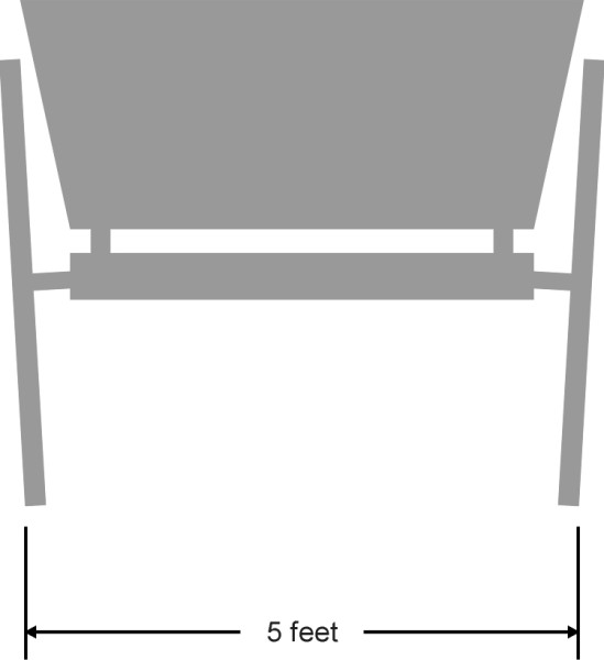
For a railway to work at all, the rails themselves must be placed a known distance apart. The separation must consistently match the wheel separation of the vehicles intended to run on them. Different gauges are used in different countries, but the most commonly used standard derives from a coalmine in the north of England. When George Stephenson began experimenting in 1814 with steam locomotives to haul trucks on the Killingworth Colliery railway, he based the track cross-section on the roadways traditionally used in Britain for horse-drawn wagons. The roadways were a minimum of five feet across (1.524 m), this being the width of a wagon measured between the outer edges of the tyres (figure 1). But Stephenson’s railway wheels had flanges, and what he needed was a gauge that specified the distance between the inside shoulders of the rails that guided the flanges. So he subtracted two inches from each side to allow for the width of a typical cartwheel tyre to give a figure of 4 feet 8 inches (1.422 m). Later, this was increased to 4 feet 8.5 inches (1.435 m) to reduce friction [9] [18]. Nowadays, the track gauge is defined more precisely as the separation between the inside faces of the rail heads measured 14 mm below the upper surfaces. The separation is usually 1435 mm but it is widened by a few millimetres on curves to ease movement [13].
Figure 1
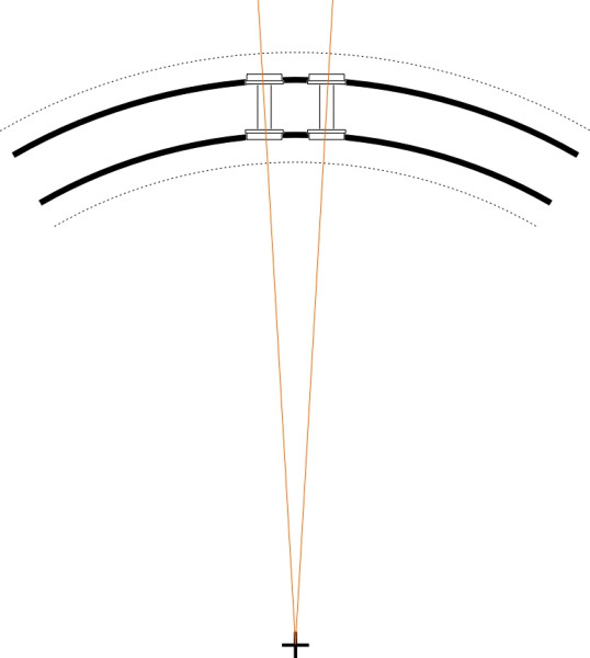
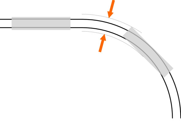
Not all railways conform to this ‘standard gauge’. There are good arguments for having a greater separation between the rails, not least the fact that vehicles travelling on a wider gauge are less likely to roll from side to side or topple over. Indeed when he built the Great Western Railway, Isambard Kingdom Brunel famously specified 7 feet 0.25 inches (2.140 m). A wide gauge permits the boiler of a steam loco to sit lower down between the wheels, which in turn lowers the centre of mass and also reduces the risk of overturning on curves. As it turned out, Brunel’s track didn’t work very well: the rails were supported on longitudinal beams and were not sufficiently well restrained laterally to preserve the track gauge. Worse, neither vehicles nor track were compatible with those of adjoining networks and eventually the company was required to convert the whole network to standard gauge - at considerable cost. Today, most non-standard systems are in fact ‘narrow gauge’, meaning less than standard gauge, because a narrow gauge improves steering on sharp curves. On a standard gauge railway, when a train encounters a sharp curve as it occasionally does in constricted locations such as London Bridge station in the UK, it must slow down almost to walking speed. The outer wheels and the inner wheels are forced to travel unequal distances, which causes them to grind along the top of each rail. And because they don’t align properly with the track (figure 2), the flanges grind against the outer gauge corner, which increases the risk of jumping the rails (we’ll have more to say about this in Section R0415 and R0314). In countries where the topography is difficult and resources scarce, small curve radii are inevitable, and with the rails closer together, the difference in path length between the inner and outer wheels is reduced, and the bogie wheelbase can be shortened to improve the angle at which the leading outer wheel attacks the rail (figure 3). Effectively, if you halve the gauge and halve the wheelbase of a bogie, you scale down the geometry of the whole system so that the minimum tolerable radius can be reduced by a factor of two without endangering the relationship between the wheel and the rail.
Figure 2
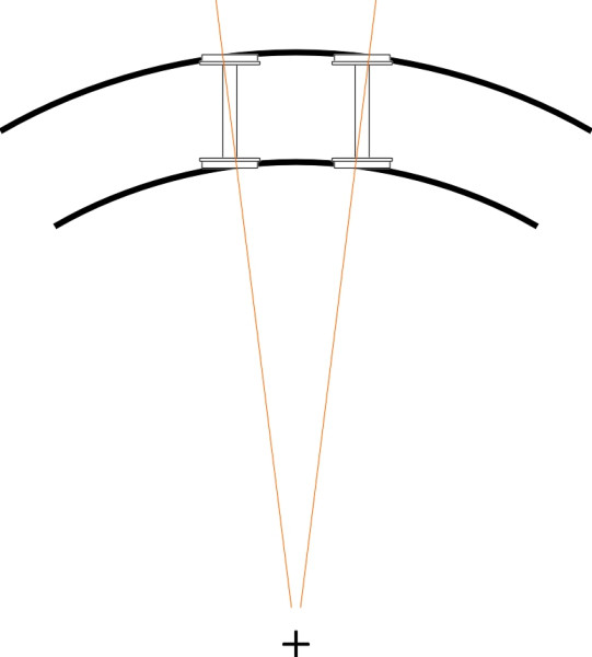
Figure 3
The vehicle and structure gauges
A narrow track gauge does not necessarily mean a narrow vehicle. Although it may seem precariously balanced, a narrow gauge railway is designed to run at a lower speed so the coaches don’t topple over on curves. Assuming that stability is not an issue, what matters is the vehicle gauge and the structure gauge, which like those for standard-gauge railways, are developed in parallel to ensure a suitable minimum clearance between the vehicle and its surroundings. The usual clearance in the UK post-nationalisation (1951) was 150 mm, which allowed 100 mm for vehicle movement on its suspension, and 50 mm for track positional and geometric errors [6].
Until about thirty years ago, it was customary for each railway company to subscribe to a fixed vehicle gauge and a fixed structure gauge that applied across any given line together with its associated branches and depots. The process was called ‘static gauging’ [6] and it required negotiation and compromise between on the one hand vehicle engineers who wanted their trains to carry the maximum payload at the highest possible speed, and the civil engineers who were trying to keep down the cost of land purchase and track construction. During the early years of the railway boom, in each country there were significant variations between lines built at different times to different standards, which were subsequently inherited by the national system. In Europe today, different vehicle gauges apply to different parts of the network. Those countries that pioneered railway construction have inherited the greatest variations, often with relatively narrow tunnels and over-bridges by modern standards. Height clearance can be a particular problem because it is determined by the needs of freight vehicles, and there is continuing pressure to increase the size of a standard container. But it’s an expensive and time-consuming operation to raise the height of a bridge, and almost impossible to raise the roof of a tunnel. In practice, it may be easier to lower the track. For example, in December 2009, the line through the Southampton tunnel in the UK was lowered by substituting a concrete slab for the ballast, which, being more stable, made gauging analysis easier and allowed for smaller clearances than would otherwise have been the case.
Figure 4
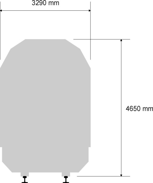
In Europe, vehicle gauges are undergoing continual revision as the national operations are brought into a common framework. Figure 4 shows the overall width and height in operation some years ago [2]. For the more recently constructed high-speed railways, the vehicle gauges are not very different, but they need a substantially greater clearance between the track centrelines because of the aerodynamic interaction between trains travelling in opposite directions, in some cases up to 4.8 m [14]. More data on vehicle gauges in different countries can be found in [24].
But the notion of a fixed gauge is becoming obsolete. Complications arise on curves, where vehicles project beyond the envelope they occupy on straight track, a phenomenon called ‘overthrow’ (figure 5). The increasing length of coaches has prompted a modified approach called swept (‘geometric’) gauging, which varies along the track, to take into account the swept paths of modern long vehicles. Special considerations apply to tilting trains, in particular the Spanish Talgo trains, which tilt around a high axis [7].
Figure 5
Even after allowing for swept paths, at any given point on the track there is still an element of risk. The rails will shift over time and may not lie precisely where the civil engineers think they are. And the vehicle themselves will roll and yaw to a degree that varies with the amount of wheel wear and the condition of the suspension, so there is always uncertainty about the relationship between the train and the track environment. The actual gap between the body shell of the rolling stock and nearby objects may vary from one train to another, and over time. Hence a fixed vehicle gauge and a fixed structure gauge require liberal clearances to allow for random variations in geometry that occur in real life. If these variations are built into the clearance dimension, this can delay innovation, for example, the introduction of softer suspensions on existing trains. Nowadays, the concept of gauging is moving towards something more sophisticated, with a computer-based gauging procedure in which the variations are explicitly modelled in a way that allows engineers to achieve a closer fit [6]. The first step is to relate the likely movements of the vehicle to the operating environment. At any given location, the kinematic envelope is calculated using a number of input parameters, and using this model it may be easier to fit new vehicles into an existing rail environment, for example, tilting trains. A further gain can be made by using simulation software to model dynamic movement of vehicle suspension.
Cant
Any moving object such as a railway coach will undergo lateral acceleration as it travels round a curve. Railway operators try to limit the acceleration so that passengers can stand and walk along the gangway without losing their balance. The target is usually 1 m/s2 or less, roughly equivalent to \(0.1g\) where \(g\) is the acceleration due to gravity. Given that the lateral acceleration is equal to the square of the speed divided by the curve radius, it is theoretically possible to achieve the target simply by making the train slow down for every curve. This is not a good idea for a high-speed railway, where instead the layout is designed with long, gradual curves that don’t force the trains to brake and thereby lose momentum. But with an existing track, the scope for improvement is limited, and if the engineer wants to raise the operating speed, the train must lean into the curve.
Figure 6
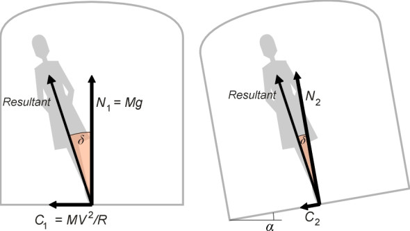
The simplest way to achieve this is to cant the track. Figure 6shows the forces acting on the feet of a standing passenger as the train goes round a left-hand curve of radius \(R\) at constant speed \(V\); the direction of motion is away from you into the paper. In the left-hand diagram, the coach stays upright and the floor horizontal. The vertical reaction \(N_{1}\) is equal to the mass \(M\) of the passenger times the acceleration \(g\) due to gravity. The centripetal force \(C_{1}\) is equal to \(MV^{2}/R\). The resultant force is directed at an angle to the vertical whose tangent is given by \(MV^{2}/R\) divided by \(Mg\), which comes to \(V^{2}/Rg\). If we were to cant the track at this angle, passengers would be able to sit or stand upright in the same way as they would on a straight track. Relative to the coach interior as their frame of reference, the transverse acceleration would be zero. Indeed, the same applies to the train, so the wheelsets would tend to settle in a central position on the track rather than push against the outer rail; they would run more smoothly and with less wear. Here is an example. Suppose that the trains are scheduled to travel at 150 km/h (41.67 m/s) on a curve of radius 2000 m. We calculate the ideal cant angle \(\alpha\) as arctan\([41.672^{2}/(2000 \times 9.81)]\) which comes to a little under 0.0883 radians, equivalent to about 5\(^\circ\). With the track canted at this angle, if you travel as a passenger you won’t feel any transverse force relative to the cabin floor and unless you look out of the window you’ll scarcely notice you are travelling round a curve.
The snag is that this only works for a train travelling at 150 km/h. Any faster, and you will experience a lateral force acting towards the centre of the curve. It will be somewhat less than the value that occurs with a level track but nevertheless you must lean inwards to compensate: there is a cant deficiency. We’ll denote this angle by the symbol \(\delta\). Any slower, and you’ll experience a net lateral force in the opposite direction: the train is tilting too far and you must lean outwards to compensate. In these circumstances, there is a cant excess, and \(\delta\) becomes negative. A cant excess can be just as much of a nuisance as a cant deficiency, because if the train is forced to halt for any reason, passengers may find it difficult to sit or stand upright. Also the inner wheels tend to jam against the rail, and if a freight train is forced to halt on the curve, it may need help to get it going again. In practice, therefore, any cant angle that is built into the track must take account of the likely variations between trains in speed and tractive power. All railway operators aim to contain the transverse acceleration for passengers to around \(0.1g\) or less, and to do this, they must work out for each curve the range of speeds at which the train can be allowed to travel.
Figure 7
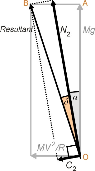
The maths is straightforward. The diagram on the right hand side of figure 6 shows what happens when the track and vehicle are canted at an angle to the horizontal denoted by \(\alpha\), expressed in radians. Note that the cant deficiency \(\delta\) is much reduced, and we would expect the transverse force experienced by the passenger within her new frame of reference to be reduced also. To find the transverse force \(C_{2}\), we must resolve \(C_{2}\) and \(Mg\) parallel to the cabin floor. Figure 7 shows the geometry in more detail. We have
(1)
\[\begin{equation} C_{2} \quad = \quad \frac{MV^2}{R} \cos \alpha \; - \; Mg \sin \alpha \end{equation}\]so that
(2)
\[\begin{equation} \frac{C_2}{Mg} \quad = \quad \frac{V^2}{Rg} \cos \alpha \; - \; \sin \alpha \end{equation}\]and since \(\alpha\) is small, to a close approximation this can be written
(3)
\[\begin{equation} \frac{C_2}{Mg} \quad \approx \quad \frac{V^2}{Rg} \; - \; \alpha \end{equation}\]Now if we want to avoid making passengers uncomfortable we must limit the transverse acceleration to a maximum of \(0.1g\), say, so the force \(C_2\)must lie within the range \(-0.1Mg\) to \(+0.1Mg\). Hence
(4)
\[\begin{equation} - 0.1 \quad \le \quad \frac{C_2}{Mg} \quad \le \quad + 0.1 \end{equation}\]and if we substitute for \(C_2\) via equation 3 and re-arrange things slightly we conclude that the vehicle speed must be limited according to
(5)
\[\begin{equation} \alpha \; - \; 0.1 \quad \le \quad \frac{V^2}{Rg} \quad \le \quad \alpha + \; 0.1 \end{equation}\]For the example mentioned earlier with \(\alpha\) set to 0.0883 radians, the lower limit is negative so the train can travel slowly and even stop without unduly disturbing the passengers. It remains to look at the upper limit, which implies a maximum speed \(V_{m}\) for the vehicle speed satisfying
(6)
\[\begin{equation} \frac{V_m^2}{Rg} \quad = \quad 0.0883 \; + \; 0.1 \quad = \quad 0.188 \end{equation}\]which in the present case with a curve radius of 2000 m leads to \(V_{m}\) = 60.8 m/s or 219 km/h.
Transverse force and cant deficiency
Let us pause for a moment and look more closely at the notion of cant deficiency. It is a notion widely used in railway engineering and one that will turn out to be useful later on. In figure 6 we pictured cant deficiency as the angle \(\delta\), the angle between the resultant force acting on the passenger’s body and the perpendicular to the cabin floor. It is the angle at which a standing passenger would lean in order to keep his or her balance without using a handhold. The forces acting on the vehicle as a whole follow the same pattern, and indeed the resultant force exerted by the track on each wheelset lies at the same angle \(\delta\) to a line drawn perpendicular to the track. Note that if the vehicle is equipped with a tilting mechanism the cant deficiency perceived by the passenger is reduced because the passenger’s frame of reference is altered; we’ll deal with tilting vehicles separately in Section R0410. However, the configuration of forces acting on the wheelset remains unchanged. In either case therefore, we can interpret the forces shown in figure 7 as the forces acting on a wheelset that carries a static load \(Mg\) travelling round a curve of radius \(R\) at constant speed \(V\) (the term ‘static load’ means the weight the axle carries when the vehicle is stationary on level track). In triangle OAB we see that
(7)
\[\begin{equation} \tan (\alpha + \delta ) \quad = \quad \frac{MV^{2}/R}{Mg} \quad = \quad \frac{V^2}{Rg} \end{equation}\]and if we substitute \(tan(\alpha+\delta\)) for \(V^{2}/Rg\) in equation 2 we get
(8)
\[\begin{equation} \frac{C_2}{Mg} \quad = \quad \tan (\alpha + \delta) \cos \alpha \; - \; \sin \alpha \end{equation}\]As it happens, both the tangent of a small angle and the sine of a small angle are approximately equal to the angle itself (expressed in radians). Also the cosine is approximately equal to 1. So when \(\alpha\) and \(\delta\) are small, to a close approximation equation 8 can be written
(9)
\[\begin{equation} \frac{C_2}{Mg} \quad \approx \quad (\alpha + \delta ) \; - \; \alpha \quad = \quad \delta \end{equation}\]In other words, expressed as a proportion of the static axle load, the transverse force acting on the wheelset measured parallel to the plane of the track is approximately equal to the cant deficiency in radians. The correspondence is not exact but it is close enough for most practical purposes. The same applies to a passenger on a conventional (non-tilting) train: expressed as a proportion of her body weight, the transverse force she perceives is approximately equal to the cant deficiency in radians. And we can carry the logic a step further: since force equals mass times acceleration, we can interpret the left-hand side of equation 9 as the acceleration experienced by the passenger or the wheelset measured in units of \(g\). This is what makes the cant deficiency notion useful to railway engineers, who use terms like ‘lateral force’, ‘transverse acceleration’ and ‘cant deficiency’ almost interchangeably. For example, if in a particular case we are told that the cant deficiency is 4\(^\circ\), its value in radians must be \(4\times\pi/180 = 0.07\)approximately. The transverse force acting on a wheelset will be equal to 0.07 times the static load, and the transverse acceleration will be \(0.07g\).
Alignment
When setting out a new railway line, the promoter will usually try to find an alignment between stations that lies as close as possible to a straight line. Other things being equal, a direct route costs less to build and provides a quicker service. But threading a railway through a densely populated area or through mountainous terrain requires difficult choices to be made. Either the track is carried on viaducts and through tunnels, which cost many times more per kilometre than construction over level ground, or the route curves around the obstacles.
Horizontal alignment
The early railway builders had available steam locomotives of limited tractive power and speed, so they avoided steep gradients wherever they could. Hence early railways did not always follow the most direct route through the landscape. Within the UK, although improvements have since been made, about half the current mileage is on curves, many of comparatively small radius between 500 and 2000 m [11]. By contrast, the lines that make up the modern TGV network in France have a minimum radius of 4000 m or more [12].
Figure 8
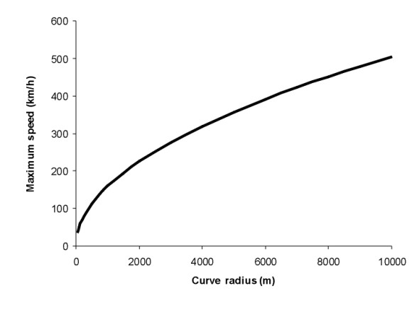
The severity of the curves on a railway line effectively sets the operating speed. If we fix the maximum lateral acceleration at \(0.1g\), roughly equivalent to 1 m/s2, together with a maximum cant of 0.1 radians, then equation 5 tells us that the maximum permissible speed \(V_{m}\) on a curve of radius \(R\) must satisfy
(10)
\[\begin{equation} \frac{V_m^2}{Rg} \quad = \quad 0.2 \end{equation}\]figure 8 shows the relationship between \(V_m\) and \(R\). If the track radius is 4000 m, the maximum speed comes to about 320 km/h, whereas if we reduce the radius to 1000 m, the speed is halved, to 160 km/h.
When the railway line is first laid out, it is advisable to include a transition on the entry to and exit from each curve, in exactly the same way that a highway engineer incorporates transition curves on high-speed roads, so that the vehicle and passengers are not subjected to a sudden change in lateral acceleration. We have already referred to the ‘rise time’ that standing passengers need to adjust, and how this is related to the jerk level or rate of change of lateral acceleration (Section G0216). Typically, a railway transition curve has the geometry either of a clothoid curve [4], or a cubic parabola [15]. The clothoid is defined by the requirement that the curvature \(\rho\) (which is equal to the inverse of the radius) increases linearly with length \(L\) measured along the centreline of the track from the start of the transition, so that
(11)
\[\begin{equation} \rho \quad = \quad kL \end{equation}\]By contrast, for the cubic parabola,
(12)
\[\begin{equation} \rho \quad = \quad kx \end{equation}\]where \(x\) is the projection of the length onto the tangent at the origin of the transition. In most cases the two give similar results, and both produce the desired effect: the cant is applied gradually along the transition section. Details of the method of calculation for the cubic parabola can be found in [15].
Vertical alignment
As well as curving to the left and right, a railway track curves up and down with changing elevation above sea level. But the variations in height are comparatively small and gradual: until recently, a fast route was expected to have gradients of no more than 1.5% [13], and for conventional tracks, even in the most difficult terrain, the grade rarely exceeds 5% anywhere in the world. There are three reasons for this. First, steel wheels have limited grip on a steel rail, a factor that particularly affects freight locomotives, which may be hauling loads weighing thousands of tonnes. In wet weather with organic debris on the rail surface, braking on a steep downhill grade can be difficult, and if halted on an uphill grade the train may fail to re-start. The second reason has to do with power. Even if there is enough grip, an uphill gradient absorbs some of the tractive power and the speed falls, which prolongs the journey time and reduces the capacity of the line as a whole. The third and final reason is that a high tractive effort raises the tension in the couplings between adjacent wagons, which on a long freight train can be a cause for concern (see Section R0204).
These considerations are less important for passenger vehicles, especially electric trains whose tractive motors have a much higher power-to-weight ratio than diesel locos. On the TGV lines recently built in France such as the Paris-Lyons line, the maximum gradient is 3.5% [12]. Presumably the trains are powerful enough to climb these grades without significant loss of speed - their momentum carries them over. However, it is important to blend the gradients using vertical transition curves in the same way that horizontal straights and curves that we mentioned earlier. Details can be found in [16].
The switchback railway
The ideal railway would run inside a tube with the air pumped out to make a vacuum. The coaches would be suspended by magnetic levitation. Since there would be no wheel friction and no air resistance, when the train was ready to start its journey, a gentle push from the stationmaster would set it moving, and on a level track it would keep moving without any power input until it reached the next station. In fact, when viewed on a large scale, such a track would follow the curvature of the earth’s surface (figure 9). It would be an efficient arrangement because the train wouldn’t need energy to climb any slopes.
Figure 9
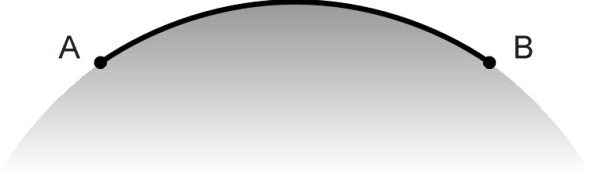
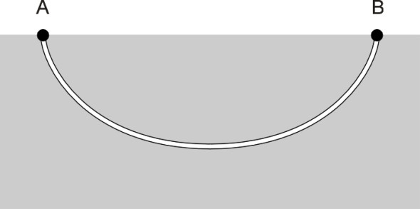
But there’s a better way. Imagine two stations A and B located at the same height above sea level. Instead of following the earth’s surface, we can make the tube follow precisely a straight line between the terminals A and B. If the terminals are a considerable distance apart, this requires a tunnel between them (figure 10). When a train is released from A it is on a downward slope and therefore it accelerates under the action of gravity, accumulating kinetic energy as it goes. Maximum speed is reached at the midpoint of the tunnel, and afterwards the speed declines as the train rises up the slope, finally coming to a halt at station B where all its kinetic energy is exhausted, without the driver ever touching the controls.
Figure 10
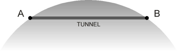
So how quickly would the train get there? It turns out that regardless of the distance, it would take just 42 minutes to get from A to B. If, for example, station A were located in the centre of Paris and station B in Wellington, New Zealand on the opposite side of the globe, a distance of about 12 700 km, the train would fall through the centre of the earth reaching a maximum speed of about 28 000 km/h, and arrive at its destination 42 minutes later. The passengers would be in free fall throughout. If on the other hand the stations were only 200 km apart the tunnel would follow a relatively gentle slope, dipping only 785 metres below the earth’s surface. For adjacent stops on the Paris Metro 200 m apart, the drop would be a little less than a millimetre - and the journey would still take 42 minutes. This bizarre concept first emerged about 400 years ago, and has resurfaced many times since. The story is told briefly by Alexandre Eremenko [21], whose notes can be downloaded from the web site listed at the end of this Section.
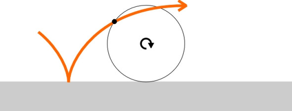
But there’s an even better way: the train will get there quicker if we make the vertical alignment dip below the straight line joining A and B. There is a particular shape of curve - the ‘brachistochrone’ - that leads to the minimum journey time, and the story of how it was discovered goes back almost as far as the gravity train concept just described. In its original form, the brachistochrone had nothing to do with transport as such, but was considered by philosophers as an interesting challenge in its own right. Although he didn’t solve it, Galileo was intrigued by the problem of how to build a ramp or slope down which a bead or marble would roll in the shortest possible time. Should the profile of the ramp follow a straight line, or should it follow a curve, and if so, what curve (figure 11)? Galileo favoured a circular curve, but in fact the solution turns out to be a cycloid, which happens to be the path traced out by a point on the rim of a circular wheel rolling along a flat surface (figure 12). Using concepts borrowed from optics, it was Johann Bernoulli who in 1897 published a proof that the cycloid represented the curve of quickest descent. From this first step emerged a whole branch of mathematics devoted to finding optimal curves or functions (as opposed to the more familiar maximum and minimum values that we learn in calculus at school). It became known as the variational calculus. A succinct review of the mathematics can be found in the notes by Alex Friere [22] and also by O’Connor and Robertson [23], both available for downloading from the web sites listed at the end of this chapter.
Figure 11
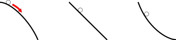
Figure 12
What we are interested in here is how to adapt Bernoulli’s cycloid to make an efficient railway, given that we are allowed to bore a tunnel to any depth we wish between two stations A and B located a distance \(L\) apart at the same height above sea level. Since tunnelling is very expensive, we wouldn’t expect this to be viable for inter-city routes, but in the case of an urban metro where the decision has already been take to go underground, the brachistochrone seems to be a promising line of attack. In fact the curve of quickest descent transforms into the railway problem if we introduce a second curve which is a mirror image of the first, place them back-to-back, and let the bead slide down the first ramp and then up the second ramp to its destination (figure 13). But here we hit a snag - three snags in fact. The slope of the cycloid is infinite at A and B, which would be difficult to arrange in practice: passengers prefer the train to stay more-or-less horizontal throughout the journey, and certainly won’t enjoy the sensation of falling vertically into a tunnel after leaving the station platform. Secondly, real trains experience both rolling resistance and air resistance and therefore the cycloid doesn’t apply. Thirdly, the nature of the ground under most cities doesn’t allow a free choice of profile: the route must avoid geological weaknesses together with obstacles such as sewers and other underground services and it may not be possible for the profile to follow a well-defined mathematical curve.
Figure 13
Nevertheless, during the railway boom of the nineteenth century, engineers made use of the principle to a limited degree. The alignment of many underground lines dips between stations so that when it leaves the platform, each train receives a little gravitational help by accelerating on a downward slope, and then it coasts for a while, and finally it climbs an upward slope that relieves the brakes of some of the effort needed to stop the train at its destination. One author has suggested that for underground trains running at 100 km/h, the dip between stations should be about 40 m [3], and indeed, the Central Line in London was originally designed with a downgrade of 1:30 for 300 feet on leaving a station, and an upgrade of 1:60 on the approach to the next [1] [10]. The ‘humpback’ profile on the more modern Victoria line is said to speed up trains by 9% and provide an energy saving of 5% [8].
Alignment errors
When building a new railway, the construction team will carefully position the track so it meets the various gauging requirements. But over time, the rails and sleepers shift away from their original positions, so if you were to choose a cross-section of the track at random you would find each rail some distance - hopefully a small distance - away from where it was meant to be.
Figure 14
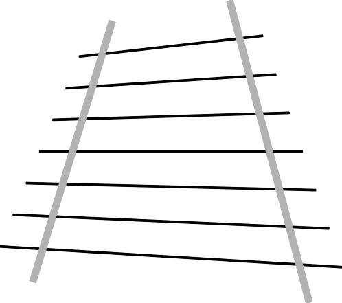
In fact, five distinct types of alignment error can occur on a railway track. The first relates to the gauge, the distance between the inside faces of the two rails. No train can run safely at speed on a track where the gauge is incorrectly set, or the inside faces of the rails are badly worn. The next two, elevation and horizontal alignment, refer respectively to the vertical and horizontal positions of the track centreline. A particularly serious form of misalignment arises when the track buckles laterally as it expands during hot weather, as it did on the UK network in August 2003 where more than 9 buckled rails were spotted in just two days. Track laid on a concrete slab is more stable but as we shall see later in Section R1602 it has other disadvantages. Next comes the cant: the tilt in the cross-section which is built into the alignment to offset lateral acceleration on curves. Finally, there is a more subtle error known as twist. If you imagine the four wheels of a vehicle bogie mounted in the bogie frame, then the four points at which you would expect the wheels to contact the rail lie in the same plane. As its name implies, ‘twist’ in the track alignment is a rotation of the kind you get if you stretch a ribbon between your hands and twist one end slightly as shown in figure 14. If you now imagine the track as a flat ribbon that is twisted slightly out of line, the four points on the rail surface where the bogie wheels would be expected to make contact no longer lie in a plane, and one wheel will be lightly loaded or even lift off the surface. This more than any other circumstance is liable to cause a derailment. For safe operation, all these types of alignment error must be kept within certain limits, and table 1 shows some typical values.
| Characteristic | Limit | Measurement base |
| Gauge | -3 mm to +10 mm | N/A |
| Rail elevation | 10 mm | 10 m |
| Horizontal alignment | 10 mm | 10 m |
| Cant | 7 mm | 10 m |
| Twist | 3.3 mm | 1 m |
In practice, the errors will vary from place to place along the line, partly at random and partly reflecting the nature of the ground over which the track is laid. Some railway lines are better than others. For example, high-speed tracks are kept in good shape compared with suburban lines, and if you look at a siding in a neglected corner of a station you will not need any surveying instruments to see the kinks and undulations in the rails. For any chosen section, the degree of variability can be quantified, and the process of measuring the errors can be automated using equipment mounted in a moving vehicle, which produces among other things a linear trace of the rail alignment [19]. As in the case of a road surface, (see Section C1603) one can express the height of the rail surface above datum as the sum of a collection of sine waves, and the sine waves themselves can be represented by a single curve known as the Power Spectral density (PSD) curve. The PSD of a railway track was first measured by Gilchrist in the UK in 1967, using a special trolley [20]. Some notional curves appear in [5].
Conclusion
An accurate alignment is desirable for several reasons. First, it reduces the likelihood of a train fouling any trackside structure. Second, it leads to a smoother ride, which makes the service more attractive to passengers. Third, it reduces the risk of a derailment, which disrupts services and can damage the reputation of the company. Finally, it produces less wear and tear on the wheels, the suspension, and the track. In a perfect world, all railways would be built to millimetre precision so that a train floats smoothly from town to town with no perceptible vibration at all. Modern track comes close to this ideal, but it’s not an easy standard to keep up: maintenance must be frequent and thorough. In order to avoid interrupting services, it is often carried out at night, and it accounts for a large proportion of the operating costs of a railway. We’ll be looking more closely at the nature of the task later in Section R1602.