The control interface

When stripped to its bare essentials, the driver’s task is to control the vehicle’s motion (a) forwards and backwards, and (b) from side to side. Forward or longitudinal movement is controlled by the brake pedal and the accelerator pedal or throttle. The driver will use one or the other to speed up or slow down. If the road is busy, the driver will also want to keep a safe distance behind the vehicle in front, and from time to time, halt the vehicle at a particular location, for example, a pedestrian crossing. Lateral movement is controlled via the steering wheel, which we’ll call the handwheel to distinguish it from the vehicle’s front wheels. Of course, a vehicle doesn’t actually move sideways, but if you turn the handwheel it will rotate or yaw about a vertical axis while its path curves to the left or right. As a result, its lateral position will shift relative to the road centreline.

Throttle and brakes

For a ship or an aircraft powered by an internal combustion engine, the throttle controls the fuel supply to the engine cylinders. It takes the form of a control lever, which if left alone, will hold its setting so the vehicle can cruise for long periods without further adjustment. The setting is calibrated in terms of engine revolutions rather than fuel flow, and the lever may be linked to a governor that holds the rpm steady when the load varies.

Road vehicles are different. As far as I’m aware, a road vehicle is the only kind of vehicle whose engine power is controlled through a foot pedal. The pedal is fitted with a return spring and needs continuing foot pressure to remain open. There are good reasons for this, but over a long journey, it’s not easy for a human to maintain a precisely targeted level of engine power in this way. In fact, the power needed to maintain a given speed varies from moment to moment according to the highway gradient, wind conditions, and the quality of the road surface. So during a typical journey, the driver will make frequent adjustments to the pedal angle, adjustments that are not necessarily reflected in the vehicle’s speed, as has been demonstrated by recording the pedal movements and the vehicle speed variations during test drives on public roads. To ease the workload, car manufacturers have developed cruise control systems that enable a vehicle to maintain a steady speed under motorway conditions without continuous input from the driver.

Compared with the throttle, the brake pedal is applied less frequently - and for a relatively short time on each occasion - but it has a more immediate impact on the vehicle’s speed. It is controlled by the driver’s right foot, the same foot that usually rests on the throttle, switching from one pedal to the other whenever the driver wants to slow down. The rate of deceleration is determined by the pressure on the pedal, not its position. Its value may reach \(0.5 g\) or more during emergency braking.

Handwheel

Of all the controls to be found in a motor vehicle, the handwheel is the most familiar, the device that children love to play with when allowed to sit in the driving seat. But this hasn’t always been so. Early cars were steered by means of a ‘tiller’ – a lever rather like the tiller on a yacht except that the handle was pivoted over the front wheels, and pointed aft rather than forward. However, tiller steering was soon discarded in favour of the handwheel, which was less likely to be knocked accidentally to one side. Also, the steering column input could be stepped down through a reduction gear, which allowed for more precise steering control. Finally, when the vehicle was at rest, the reduction gear enabled the driver to swivel the front wheels of the vehicle more easily, an important requirement as vehicles grew heavier over subsequent decades. Today, the geometry is arranged so that the torque increases (a) as the steering angle increases, and (b) as the vehicle speed increases; this warns the driver against abrupt or extreme steering actions.

Instrument panel

A modern vehicle is equipped with electrical and mechanical subsystems distributed around the chassis. They are linked via a communications network to the instrument panel, where the control switches that convey the driver’s ‘on-off’ commands to each individual device are located, together with dials and warning lamps that return information about its status. The operation of the controls themselves is simplified to the point where drivers can manage them without much conscious effort.

In addition, the instrument panel provides access to a range of information and entertainment functions that are not related to vehicle control, including a satellite navigation system, the climate control system, radio, CD player, and hands-free cell phone. To activate a function while on the move, the driver must (a) remember which control is which, (b) find the control, and (c) choose the desired setting (e.g., choose a radio station). The search and selection process may last for several seconds, potentially diverting attention away from the driving task long enough for a crash. Researchers have drawn attention to the risks involved, and called for gadgets in the car to be designed in a different way from gadgets in the home [15]. However, specialists agree that even a clever design cannot redeem the cell phone. Using a phone (hands-free or otherwise) is not compatible with the driving processs because having one’s eyes on the windscreen is not the same as having one’s attention on the road [18].

Driving tasks

Now let’s consider the operations that drivers perform using the throttle, brakes and handwheel. We’ll divide them into two groups. Those in the first group are the simplest: they are reflex actions carried out continually during the journey, in which the driver adjusts the speed or steering angle to keep the vehicle moving steadily along its designated lane without hitting anything. Those in the second group are consciously planned manoeuvres, for example, turning at a junction. Here, the driver assesses the road layout, decides what to do, then performs a number of actions in quick succession (they probably include checking the mirror, looking out for pedestrians and other vehicles, braking, changing gear, and turning the handwheel). These two different types of driving task seem to require different skills and different levels of concentration.

Lane-keeping

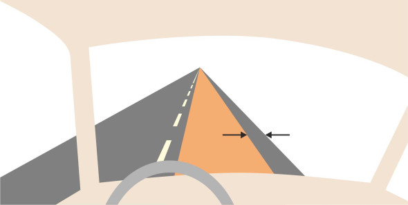
We’ll begin with one of the most basic tasks in the first group, which is to control the lateral position of the vehicle on the highway. Imagine you are driving along a two-way rural road in a country where people drive on the right. There are no sharp bends, only shallow curves and the occasional straight section. If at any moment your car seems too close to the kerb, you turn the handwheel a little to the left (figure 1). If it’s too close to the carriageway centreline, you turn a little to the right. The adjustments might be described a tracking process. It involves a feedback loop, in which your position, like the temperature in a thermostatically controlled hot water system, zigzags between acceptable limits on either side of the ‘target’ position. In this way, you can travel for long distances without consciously thinking about the road layout, and the steering controls of a modern car allow you to keep your vehicle within a few centimetres of your target.

Figure 1

Cornering

On shallow curves and straight road sections, the task we’ve just described requires no planning or forethought. Manoeuvring round a sharp bend, or cornering, is different. Here, the driver must judge the sharpness of the bend, reduce speed, and mentally plot a course through the bend in advance. As explained in Section C0415, on a modern road the geometrical layout usually includes a transition curve at the entry to each bend, followed by a curve of constant radius, then another transition curve at the exit. The transition curves enable the driver to change the vehicle’s speed and steering angle gradually, and so avoid sudden changes in the centripetal forces that act on the vehicle suspension and passengers. In such a case the operation breaks down into four stages.

1. Approach: Change gear, braking.
2. Entry transition: The driver turns the handwheel away from its straight-ahead position, possibly while continuing to brake. The vehicle rotates or yaws at a progressively increasing rate, while the centripetal force builds up gradually to a maximum.
3. Constant radius: Theoretically, during this stage the yaw rate and centripetal force are constant (we have already touched on the dynamics of the vehicle on a curve of constant radius in section C0418, where we used a mathematical model to demonstrate key aspects such as ‘oversteer’ and ‘understeer’).
4. Exit transition: The driver ‘unwinds’ the steering and begins to accelerate. The yaw rate and centripetal force fall away gradually to zero.

On the approach to a bend, it is easy to misjudge the curvature and enter the transition too fast, so drivers tend to reduce speed to a level that leaves a margin for error. Once on the transition curve, the vehicle will continue to slow down because the resistance of the tyres increases when travelling on a curved path. The driver will continue to assess the severity of the bend and if necessary, make a further adjustment. One specialist [7] has drawn attention to the importance of yaw velocity and lateral acceleration as cues during stages (ii) and (iii). Yaw is just a change in the direction in which the vehicle is pointing, so that distant landmarks appear to move across one’s field of vision. Next, the driver senses the lateral acceleration as the slip angle of the tyres builds up (C1717), developing a centripetal force that deflects the car away from its original (straight line) trajectory and guides it round the curve. From these cues, the driver tries to judge the severity of the bend and how much grip is left in reserve, but they don’t occur simultaneously: the lateral acceleration lags behind the yaw. Once the vehicle enters stage (iii), things settle down. It’s the transient conditions at the beginning and end of the curve where the cues are out of phase.

The cues can actually contradict one another if the driver switches between lanes on a multi-lane highway when trying to avoid a collision. Imagine you are driving along a motorway and need to move to the neighbouring lane on your left. You turn the handwheel, the vehicle yaws to the left, and then begins to move across. You feel a lateral acceleration against your right hip and shoulder. Halfway through the manoeuvre, you begin to rotate the handwheel in the opposite direction. But owing to the complex transient behaviour of the vehicle mass and suspension, the lateral acceleration continues until after you have ‘unwound’ the steering and after the vehicle starts to yaw to the right. At this point, the two cues are delivering contradictory messages [7], and it seems that drivers find this disconcerting. In fact, manufacturers use ‘slalom’ manoeuvres when testing new models, presumably to expose any quirks in behaviour that might take customers by surprise. But a car can never be entirely fool-proof, as demonstrated by the widely publicised roll-over that occurred when two Swedish journalists tested the new Mercedes-Benz A-class vehicle just before launch in 1997 [2].

Speed

As with lane-keeping, controlling the vehicle’s speed is – on paper - a simple feedback process. We assume the driver checks from time to time whether the vehicle’s actual speed \(V\) is close to a notional target. If not, the driver speeds up or slows down as appropriate, by pressing harder on the throttle pedal, or by releasing it, or by applying the brakes. However, it is quite hard to adjust \(V\) within narrow limits because the foot pedals are blunt instruments – they don’t provide anything like the same degree of control as the handwheel.

For the moment, we’ll concentrate on the target rather than the adjustment process itself. The driver does not necessarily quantify the target in kilometres per hour. Some drivers look at the speedometer quite often, others rarely, and some prefer not to look at it at all, perhaps because this involves a change of focus and takes attention away from the road ahead. For much of the time, drivers rely on sensory cues such as engine noise, tyre noise, and aerodynamic wind noise, together with vibration transmitted from the road surface through the tyres and suspension. In fact, it has been suggested that a smooth, quiet ride isolates the driver from the road environment and reduces awareness not only of speed but also of road hazards such as a bend in the road ahead [19].

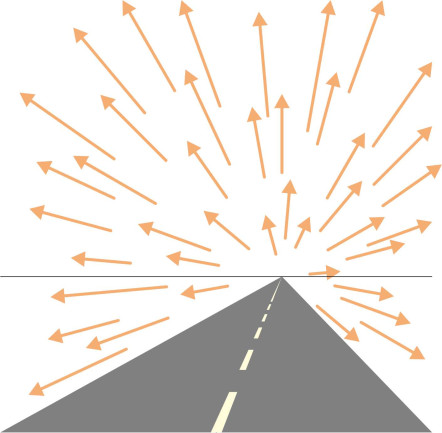
Other important cues are visual ones: motion changes the way we see our surroundings. Imagine you are sitting in the front seat of a car travelling along a straight road, looking forward through the windscreen. Different parts of the landscape seem to be moving in different directions, expanding radially from a point directly ahead (figure 2). When you look to the right or left, nearby features such as trees and fences appear to move past more quickly than distant ones. The closer the object, the more dramatic the impression of speed. The impact of the visual cues varies not only with the speed of the vehicle, but with the nature of the landscape. For example, on a narrow country lane, if there are trees and hedges close to the roadside, they will appear to be rushing past, and will reinforce the driver’s awareness of speed. Similarly on a narrow urban street. But on a wide road, the verges and hedgerows are further from the driver’s line of vision, and have less impact. As a result, one might expect drivers to feel less inhibited, and therefore drive faster.

Figure 2

In addition, the driver’s awareness of speed is affected by the speed of other vehicles nearby. Imagine you are driving along a motorway in open countryside. A platoon of vehicles in the neighbouring lane is the dominant feature in your visual field. The platoon provides a new frame of reference that is moving along the road at roughly the same speed as your car. In this new frame of reference, your vehicle appears to be standing still, or if the neighbouring cars are moving faster, it may even appear to be moving backwards. In a situation of this kind, it is tempting to imagine one is being left behind, and to increase one’s speed accordingly. The effect is stronger in foggy weather, when the cues provided by roadside features almost disappear. Under these conditions, drivers tend to underestimate their speed, and also to drive too close to the vehicle in front [14].

Speed perception is an important factor in road safety: although the relationship is a complex one, in general, both the frequency and severity of road crashes increase with the average speed of vehicles in the traffic stream. Also, fuel consumption and greenhouse gas emissions increase roughly as \(V^2\), and on a level road such as a motorway, fuel consumption is minimised at a cruising speed in the region of 50 mph (80 km/h).

Safe spacing

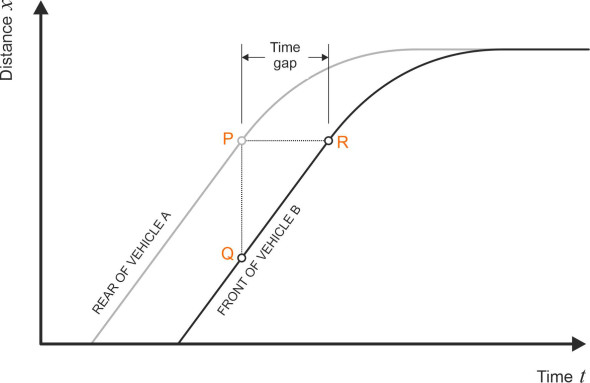
‘Tail-gating’ is a common phenomenon on high-speed roads. Imagine that vehicle A is being followed closely by vehicle B. They are mechanically similar and their minimum stopping distances are equal. We want to know the minimum time gap that will enable driver B to avoid a collision if the lead vehicle suddenly brakes to a halt. One can represent the motion of a vehicle through its trajectory, a line on a graph showing how its position along the road varies over time. Distance is usually measured along the vertical axis, and time along the horizontal axis, so that the slope of the line at any point equals its velocity. The solid grey line in figure 3 shows the trajectory of vehicle A – specifically the rearmost point of the vehicle body, while the black line shows the trajectory of vehicle B, in this case, the nose rather than the tail. The problem arises when the rear of vehicle A reaches point P, where the driver suddenly applies the brakes and carries out an emergency stop. Driver B does not react straight away, so the trailing vehicle continues for a short while at constant speed: the last possible moment for the driver to start braking is when the front of vehicle B also reaches P. Hence, the time gap must be sufficient for driver B to perceive what is happening and hit the brake pedal. Any less, and there will be a collision. Therefore in principle, the minimum safe time gap is equal to the driver’s response time, typically a little under 2 seconds.

Figure 3

In practice, highway authorities recommend a larger value, to allow for variation among the driver population and for other contingencies. There has been much discussion about how large the recommended time gap should be. Some suggest a minimum of 2 seconds, others 3 seconds (see for example [3]. All suggest a larger gap in bad weather, and in principle there are other circumstances one might wish to allow for, including the possibility that (a) vehicle B is moving faster than vehicle A when the latter starts to brake, (b) vehicle B’s braking performance is inferior to that of vehicle A, and (c) being momentarily distracted, driver B is not paying attention to what is happening on the road ahead. Note also that a 2s or 3s gap doesn’t provide a sufficient margin if vehicle A itself is involved in a collision and stops more abruptly than it would under a controlled braking manoeuvre.

Let \(T_B\) denote the time gap adopted by driver B. Ideally, she or he will aim for a ‘target’ position behind the lead vehicle consistent with this time gap, and using the accelerator and brakes, manoeuvre towards it and remain there. In principle, there are two ways that a driver can establish where the target lies. The first is to wait until the lead vehicle passes a fixed landmark such as a traffic sign, and to adjust the speed of the trailing vehicle so that it passes the same landmark \(T_B\) seconds later. This is the method recommended by the UK Highway Code. The second method is to convert the time gap into a distance gap: a two-second time gap is equivalent to a little over 0.5 metre for every 1 km/h in speed, so that a speed of 100 km/h equates to a time gap of 50 metres. The task has now transformed into one of judging distances.

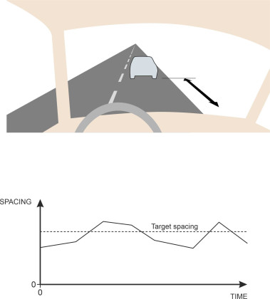
In practice, one suspects that drivers don’t consciously think in terms of time gaps measured in seconds, or distance gaps in metres, but instead, wait until the vehicle ahead looms uncomfortably large within the field of view. Whatever the strategy, assume that you are driving car B and that you have decided on a target position behind vehicle A. How you might move towards it? The foot-pedals don’t allow for very precise control, so you will converge on your target by applying a series of corrections (figure 4). If you seem to be lagging behind, you press the accelerator for a while. If you seem to be too close, you lift your foot off the accelerator for a while, and possibly switch to the brake pedal. Again, as with lateral placement and speed control, the process can be pictured as a feedback loop but with considerably larger fluctuations around the target.

Figure 4

Traffic

As vehicles move about on the road network, they interact with one another, sometimes cooperating and sometimes competing for space. Their paths cross, slower vehicles get in the way of faster ones, and there is an awkward compromise between the needs of car users and those travelling by other means, especially on foot or by bicycle. Traffic flow is a collective social phenomenon. It is a complex subject and we won’t go into detail here. Instead, we’ll round off this Section by taking a brief look at vehicle movement along an uninterrupted section of highway, treating it as a mechanistic process in which drivers all follow the same rules: our aim is to show that there is a limit to the volume of traffic it can handle. Then we’ll switch to another topic, and stepping back to view the network as a whole, compare the safety of road travel with that of other modes.

Flow

A road has many functions, but for the moment, we are interested in its ability to deliver a particular commodity – travel. The amount of travel is measured in vehicle-kilometres, and for a fixed length of road with no intermediate access points or egress points we can gauge it in terms of a simple proxy: the number of vehicles passing any particular reference point per unit time, in other words, the traffic flow. In theory, if vehicles follow one behind the other at regular intervals \(T\) along a single traffic lane, the flow will be \(1/T\) vehicles per unit time. If \(T\) is in seconds, this works out at \(3\ 600/T\) vehicles per hour. Denote the average length of vehicles in metres by \(L\), and assume they are travelling at a uniform speed \(V\) metres per second. Because of its finite length, the vehicles will take an average time \(L/V\) seconds to clear the reference point, and if we assume that each driver allows a 2 s time gap from the vehicle front to the rear of the vehicle ahead, then the mean time interval between successive vehicles will be \(L/V + 2\) seconds. Then the flow \(q\) of vehicles will be

vehicles per hour. If the average length of the vehicles is 5 m, and they travel at a speed of 80 km/h, then \(L/V\) is 0.225 s and the flow comes to roughly 1620 vehicles per hour.

However, this is a hypothetical scenario. In reality, the vehicle lengths, speeds, and spacing vary from one vehicle to the next, and small fluctuations in the speed of an individual vehicle can make the flow unstable. More than fifty years ago, researchers investigated rear-end collisions on motorways that were growing in frequency as traffic levels increased over time. Let us return briefly to the ‘safe spacing’ scenario in which vehicle B is following vehicle A along a single traffic lane, and imagine that instead of coming to a halt, vehicle A slows down for a while and then resumes its original speed. As shown in figure 5, vehicle B is a little too close behind, and must brake harder than vehicle A to restore a safe time gap. Behind vehicle B, a third vehicle C is also travelling a little too closely to the vehicle in front, and the driver has to brake harder still. If all the spacings between the vehicles upstream are too small, eventually one of them must come to a halt, and from that point on, a queue builds up, with vehicles continually arriving at the rear, working their way through the queue, and leaving at the front, so that the queue moves rearwards along the carriageway as it grows in size. Figure 6 is a simplified representation of what happens on a large physical scale. Each vehicle is shown as arriving at speed \(V\), stopping abruptly for a while, and then leaving the queue at the same speed. In reality, there should be curves between the straight-line segments to reflect the periods of braking and acceleration.

Figure 5

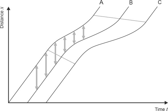
Figure 6

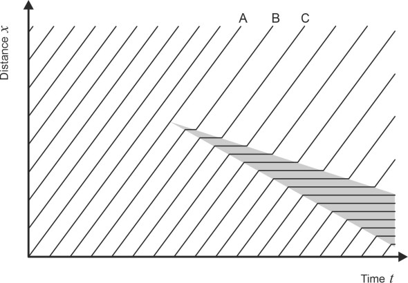
It is one of the characteristic features of congested road traffic that drivers maintain a larger gap when accelerating away from a standstill than they do when decelerating to a halt. It follows that the time interval between successive vehicles leaving the queue is greater than the time interval between vehicles entering it, and in consequence, the outflow is less than the inflow: the queue itself acts as a bottleneck. Once it has formed, two things happen. First, the rate at which vehicles can pass along the road falls, and will not recover until the demand eases off and gaps appear among the vehicles arriving upstream. Effectively, the capacity of the road to serve traffic is reduced. Second, if we denote the time elapsed since initial disturbance as \(t\), the cumulative delay to vehicles grows as \(t^2\) - the delayed vehicles are represented by the shaded area in figure 6.

Well over fifty years ago, researchers became interested in the breakdown of traffic flow, and developed mathematical models to account for it. A useful overview of their results can be found in [5]. Among the contributors was a prominent physicist who drew an analogy between vehicle motion and fluid flow along a pipe, picturing the queues as shock waves travelling along the highway [11]. Others were specialists in a discipline known as operational research, and focussing on the motions of individual vehicles, they modelled the acceleration of each vehicle at any given moment as a function of its time or distance gap [8]. Eventually, models of this kind led to practical computer control systems that could detect incipient queues and impose measures to damp down the shock waves. Among the control measures were traffic signals that temporarily halted flow entering the road at access ramps upstream, and variable speed limits [6].

Safety

Driving a car not like driving a train or a ship. The challenge lies not so much in its mechanical complexity, but in the road environment – the density of hazards, the frequency of ‘conflicts’ among different kinds of road user, and the constant level of vigilance needed to avoid a collision. The risk is offset partly by the car’s rubber tyres and the way they engage with the road surface: the grip provided within each contact patch enables the driver to apply relatively large control forces so the vehicle can brake sharply and manoeuvre around obstacles. Nevertheless, casualty levels among road users remain a cause for concern [20].

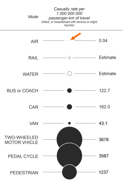
It is interesting to compare the risks incurred by road users with those attached to other modes of travel. The casualties alone don’t tell the whole story, because people cover a lot more distance by road than they do by any other means: a more useful measure is the casualty rate per billion kilometres of travel, say. I haven’t been able to find any data on this at the global level, but annual figures for the UK are shown in figure 7, averaged over the period 2010 – 2019 [4]. Note that for Rail and Water, accurate estimates of the casualty rates are not available for this period, and I have inserted ballpark estimates instead. There is a very large range of variation: compared with air passengers, cyclists and motorcyclists are over a hundred thousand times as likely to be killed or injured for every kilometre of travel. They are followed by pedestrians and car passengers, for whom the risk is around four thousand times as great.

Figure 7

Road collisions have been described as random multi-factor events, so that any given accident may be the outcome of several contributory factors. So it is not easy to account for the wide range of variation in casualty rates, and the data are open to misinterpretation. Some of the differences, particularly the high casualty rates for cyclists and pedestrians, may be attributed to exposure: if you move slowly, or in a busy environment, you take longer to cover each kilometre of travel and are exposed to more potential collisions. If the risks are quoted in terms of casualties per unit time spent in travel, the range of variation turns out to be a lot less. In addition, when a car hits a pedestrian, it is the pedestrian who is more vulnerable to injury. There are other sources of variation too, all of which influence the behaviour of the person who is controlling the vehicle. They are (i) how the user perceives risk together with the risk the user is prepared to tolerate, (ii) the level of training the user is required to undertake before being allowed to take control, and (iii) how the traffic rules are enforced, all of which vary among different modes of transport.

Coda

At present, the prospects for improving road safety seem bleak. Although casualty rates are falling in many countries, traffic levels are growing faster in others, so that globally, the total number of casualties continues to rise. However, technology may offer a solution. There are practical devices intended to alert the driver to potential risks, and others that will actually intervene and take action on the driver’s behalf, for example by applying the brakes. Among the best-known are adaptive cruise control (ACC), and its more sophisticated derivative, cooperative adaptive cruise control (CACC) in which communication takes place between vehicles. All relieve the driver of some of the burden on high-speed roads.

Ultimately, the question is whether ‘intelligent vehicles’ will be able to take full responsibility for the driving task. Autonomous vehicles have been trialled on the public road network for some time, but always with a human driver at the wheel ready to take over if anything goes wrong. At this stage, there remain a number of obstacles, but they are social and legal ones rather than technical ones: it is not yet clear who should be liable if the vehicle is involved in a crash. Not surprisingly, questions of this kind raise serious issues for the stakeholders: automobile manufacturers, law enforcement agencies, insurance companies, and highway authorities [1] [12]. On the other hand, given the present rate of progress in the field of artificial intelligence (AI), it’s conceivable that the next generation of intelligent vehicles will deliver passenger-miles of travel at a lower risk level than human drivers today. They won’t be 100% risk-free, but in principle they will be averse to risk, tireless, and therefore more reliable than humans, and if fewer lives are lost, they will perform a valuable role. This assumes of course that passengers will put their trust in a machine. And the machine won’t be programmed to avoid every possible hazard, because not all hazards can be foreseen and averted. Instead, it will advance by ‘machine learning’ in much the same way as humans do, with one priceless advantage: the experience of each vehicle will accumulate over each kilometre of travel, and shared among the fleet.