The brush model

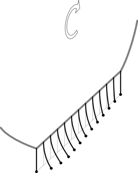
The brush model pictures the wheel as a rigid disk with bristles sprouting from the rim (figure 1). There is only a single line of bristles, and these bristles are taken to represent the whole width of the tyre tread. Each bristle acts as an elastic spring whose tip is in contact with the road. The tip can deflect in any direction, forwards, backwards and sideways across the road surface, but it resists with a force that is proportional to the deflection, in roughly the same way that the carcass of a pneumatic tyre will resist distortion under various kinds of load. For example, to represent cornering behaviour, the bristles are assigned a lateral stiffness of \(c\) per unit length of tread so the lateral deflection \(\nu\) is proportional to the lateral shear force \(q_y\) per unit length of tread. Both are measured positive to the right. The shear force and the deflection are related by the formula

The model can also be used to explain the way the tyre grips the road under braking, in which case we replace \(q_y\) with a longitudinal force \(q_x\) in equation 1, which is now taken to represent longitudinal deformation so the coefficient \(c\) represents longitudinal stiffness. In one form or another the brush model has been arouns for over 50 years, and you will find a brief summary of its development in [3]. In this Section we will use it to predict the pattern of shear force on the tyre contact patch when the vehicle is carrying out three different types of manoeuvre: (a) free rolling, (b) cornering and (c) braking. We’ll start with the ‘free rolling’ case.

Figure 1

Free rolling

When a vehicle is rolling freely along the road in a straight line at constant speed, you would think that apart from normal pressure on the contact patch that arises from the weight of the vehicle pressing on the road, there would be no other forces acting on the tyres. But owing to various forms of rolling resistance there must be a net shear force on the contact patch that opposes the vehicle’s motion. There is also the matter of carcass distortion: in Section C2019 we saw that when any given element of the tread enters the contact patch it slows down because the straight line distance between the leading and trailing edges is less than the corresponding distance measured around the unloaded tyre perimeter. This implies a compression of the tread surface and hence a shear stress that builds up and relaxes again when the tread element leaves the contact patch at the trailing edge. In other words, the tread ’creeps’ over the road surface.

Figure 2

It is possible to derive a formula for the relative movement or creep between the tread and the road as a function of its position within the contact area, and plot its longitudinal profile. To do so, we must make an assumption about the speed with which the tread element is moving at each point, and for want of anything better we’ll retain the sliding spoke constraint introduced in Section C2019. As before, rolling contact is viewed as a process in which the axle is stationary and the road passes underneath from right to left at speed \(V\) given by

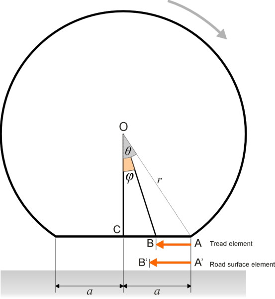
where \(r_e\) is the effective rolling radius and \(\Omega\) the angular velocity of the wheel, assumed to be constant. Denote the half-angle subtended by the contact patch at the axle centreline by \(\theta\). We choose a single tread element, picture it as an elastic bristle sprouting at right-angles from the tyre carcass to touch the road surface, and consider its progress through the contact patch assuming that the carcass can deform radially but not otherwise. The position of the bristle at any given moment is measured along the \(x\)-axis whose origin lies in the middle of the contact patch under the axle centreline. Since the tip of the bristle and its base are moving at slightly different speeds we denote their positions using two different names: \(x_t\) and \(x_b\) respectively. The time origin is set so that the bristle in question enters the leading edge A of the contact patch at time \(t=0\) (figure 2). Note that on entry, the bristle must be unstressed so \(x_t\) and \(x_b\) must be equal and in fact \(x_{t} = x_{b} = a\). After time \(t\) the base of the bristle has moved from A to B: its position at any moment can conveniently be derived from the angle \(\phi\), whose value decreases at a constant rate according to

and in turn we can write

where \(r\) is the unloaded tyre radius as defined in the previous Section. Meanwhile the road surface is moving from right to left at constant speed \(V = r_{e} \Omega\), and it carries the tip of the bristle from \(\textrm{A}'\) to \(\textrm{B}'\), a distance equal to \(r_{e} \Omega t = r_{e} ( \theta - \phi )\). The position of the tip \(x_t\) measured along the \(x\)-axis after time \(t\) is therefore given by

The deflection \(\nu\) of the bristle tip relative to its base is then \(x_{t} - x_{b}\), so

in which a positive value indicates the the bristle is bent forward in the direction of motion. If we substitute \(r \sin \theta\) for \(a\) this can be written in the slightly neater form

The final step is to convert the bristle deformation into a longitudinal force \(q_x\); this is just the right-hand side of equation 7 multiplied by the stiffness coefficient \(c\) thus:

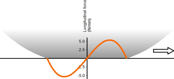
The value of \(q_x\) at each point within the contact patch can now be plotted as a function of distance \(x\) measured forward from the contact patch centre. A graph showing the resulting profile appears in figure 3 for a tyre of (unloaded) radius 0.3 m resting on a contact patch of length 0.185 m from leading edge to trailing edge. To comply with the sliding spoke constraint, the effective rolling radius is calculated from equation 5 in the Appendix to Section C2019, which yields a value of 0.2951 m. The peak towards the right hand side of the graph represents the shear stress in the front half of the contact patch, which acts on the tyre in a forward direction. The trough towards the left hand side shows a shear stress acting on the rear half in the opposite direction. Under the rather simplistic assumptions on which the model is based, the two components of shear stress cancel each other out, and there is no net force on the tyre. In practice of course, the rearward force would be the larger of the two, reflecting a net rolling resistance.

Figure 3

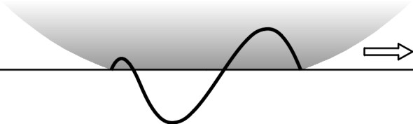
How does the curve compare with the distribution of shear force on a real tyre? Several experiments have been carried out over the years (for example [2], [5]) that point towards a distribution that is more complex than the one shown in figure 3. First, the stress profile is not constant across the width of the tyre. Second, while the profile at each shoulder is broadly similar to the one shown in figure 3, the profile in the central region often displays two reversals of stress between the leading and trailing edge as shown schematically in figure 4. However, in free rolling the longitudinal forces are relatively small and appear to be sensitive to the precise structure of the carcass and tread. In what follows, we turn to a different situation, in which large external forces are applied to the wheel that greatly alter the stress profile.

Figure 4

Shear stresses in cornering

When a vehicle is driven round a curve, the road surface applies a sideways friction force to each tyre that deflects the vehicle and keeps it on its curved path. The brush model provides a way of estimating how the lateral force might be apportioned among different parts of the contact patch on any given tyre. We shall take our lead from [1] and assume that the normal pressure is uniform along the whole length \(2a\) of the contact patch. Therefore, if the wheel load is \(P\) the normal contact force \(p\) per unit length of contact will be given by

Let us picture the vehicle from above, with its path curving to the left. Figure 5 shows a particular wheel moving from left to right across the page. It is pictured as a thin disk with a single ring of bristles round its perimeter, so the diagram shows only the central plane AB of the contact patch, which is aligned with the \(x\)-axis and has total length \(2a\) measured from the leading edge to the trailing edge. The lateral force exerted on the bristles by the road surface bends them to the left and hence the wheel doesn’t actually travel in the direction it is pointing but at an angle \(\alpha\) to the \(x\)-axis. The angle \(\alpha\) is called the ‘slip angle’. The coloured arrows represent the bristles in plan view, and you can see that when a bristle first enters the contact patch its sideways deflection is zero, but it increases linearly until it reaches a certain threshold, levels off, and thereafter remains constant.

Figure 5

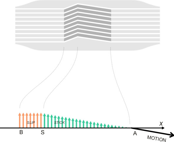
What is happening here? Within the sector from A to S, the bristles adhere to the road surface but under increasing lateral strain. At the threshold point S, the lateral force exceeds the available friction and the tip of the bristle slips sideways across the road surface. We assume here that the coefficient of sliding friction is the same as the static value \(\mu\), so aft of the threshold point, the lateral force per unit length of tread is held at the value \(\mu p\). If we label the threshold deflection \(\nu_m\), then because the stiffness of the bristles \(c\) per unit length is by definition force divided by deflection, we can write

and therefore

At this point we must pause and consider two distinct cases.

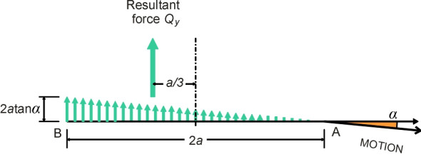
Adhesion only

If you drive round a shallow curve without putting a great deal of lateral force on the tyres, the slip angle \(\alpha\) will be small. Indeed if it is less than \(\nu_m/2a\) you can see from figure 5 that the whole of the contact patch adheres to the road surface without any slip. Hence the diagram must be re-drawn as shown in figure 6. The deflection now grows continuously from zero at the leading edge to the value \(2a\textrm{tan} \alpha\) at the trailing edge, so the mean lateral deflection is \(a\textrm{tan} \alpha\) and the mean lateral force \(ca\textrm{tan} \alpha\) per unit length of tread. The total lateral force is then given by

and because the force distribution is triangular, the resultant is located two-thirds of the way along the contact patch at a distance of \(4a/3\) from the leading edge. It therefore lies behind the axle centreline, which has a significant influence on the way the car handles. As will be explained later in Section C1405, the resultant force on the tyre creates a self-aligning moment that tends to swivel the wheel back into the ‘straight-ahead’ position, a useful stabilising effect known as ‘castor’. The lever arm about the contact patch centre is called ‘pneumatic trail’ and its value according to this analysis is given by

The value of the self-aligning moment \(M_z\) is just the product of the lateral force \(Q_y\) and the pneumatic trail, thus:

In practice, real tyres have a larger pneumatic trail than equation 13 suggests, typically around \(0.5a\) [4].

Figure 6

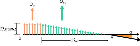
Mixed adhesion and slip

During a more severe cornering manoeuvre, the slip angle will be larger, and the lateral force acting on the rear part of the contact patch will reach the maximum value that friction with the road surface can sustain. This threshold value is \(\mu p\) per unit length, and when it is reached, the rear part of the contact patch will slip sideways while the forward part maintains regular contact. This is the configuration shown earlier in figure 5. It is re-drawn in figure 7 with the lateral force \(Q_y\) broken down into two separate components. The first one, labelled \(Q_{ya}\), is the resultant of the triangular stress profile acting on the ‘adhesion’ part of the contact patch and the second, labelled \(Q_{ys}\), acting on the ‘slip’ region. The various dimensions shown in the Figure are all related to the position of the frontier between adhesion and slip, which we locate at a distance \(2a \lambda\) from the leading edge where \(\lambda\) is a dimensionless parameter whose value can be fixed anywhere in the range from 0 to 1. It can be used as a convenient proxy for the slip angle \(\alpha\), to which it is linked via the formula

We can now work out expressions for the two lateral forces. Without going into detail, they come to

and

When they are added together, we get the total lateral force as

The self-aligning moment is given by

and finally,

Figure 7

Plotting the results

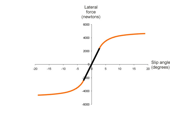
The final step is to plot the lateral force and self-aligning moment as a function of slip angle for a particular tyre. We’ll use the following parameter values by way of illustration: \(a\) = 90 mm, \(P\) = 5 kN, \(c\) = 3 MPa, and \(\mu\) = 1.0. Let’s look at the lateral force first (figure 8). The central part of the curve passes through the origin and is coloured in black. It represents adhesion-only behaviour up to the slip threshold while the remainder in red represents mixed adhesion and slip. Within the central section the lateral force is roughly proportional to the slip angle. Moving up the curve from the origin to the right we see that when the slip threshold is reached, while the total force continues to rise, it does so less quickly, and eventually levels out with the slip angle approaching 90 degrees.

Figure 8

Next we turn to the self-aligning moment. Interestingly, while it rises with slip angle from the origin in much the same way as the lateral force (figure 9), it reaches a peak when the tyre approaches the slip threshold and then declines for higher slip angles. This reflects how the steering feels when you drive your car into a bend at high speed: as detailed in Section C1405, you must tug the handwheel quite hard at first, but when the tyres start to slip the resistance suddenly dies away and steering feels ‘loose’. Some regard this as a useful warning that the tyres are close to the limit of adhesion (assuming of course that the driver is alert and knows what to do next).

Figure 9

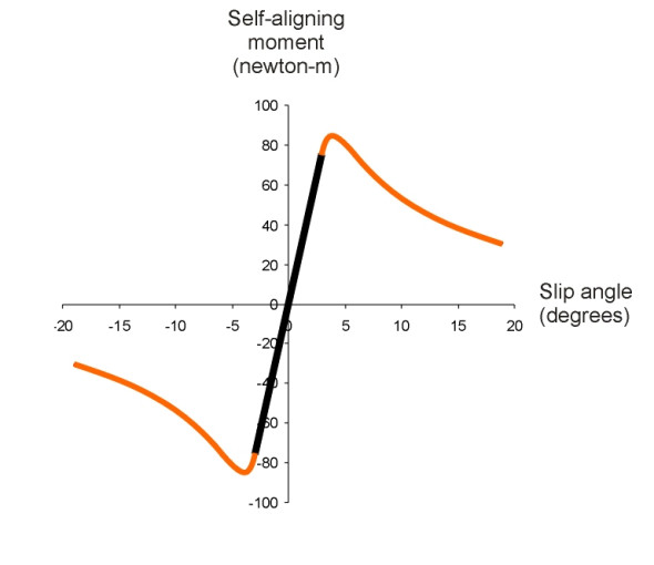
Figure 10

Shear forces in acceleration and braking

We saw earlier that when a pneumatic tyre is rolling freely, there is a mismatch between the speed at which each tread element moves through the contact patch and the speed of the road element on which it rests. The disparity leads to tangential stresses between the tyre tread and the road in the fore-and-aft direction, with one or more stress reversals between the leading and trailing edges. But when the driver applies the brakes, these stresses are swamped by larger ones that are directed uniformly rearward along the whole contact patch. The same applies in reverse to a driven wheel when the driver accelerates, but we’ll only consider the braking case.

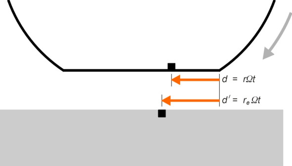
To begin with, it helps to remember that if a wheel is rotating freely with angular velocity \(\Omega\), the tread must pass through the contact patch at a speed relative to the axle centreline equal to \(\Omega r\) where \(r\) is the unloaded radius of the wheel. Ignoring any small variations arising from extension or compression, we’ll assume this speed is constant throughout the contact patch. Now when a braking force is applied to the wheel, the tread creeps forward along the road surface and the effective radius \(r_e\) differs considerably from \(r\). Let’s watch a tyre tread element as it moves through the contact patch, starting with the clock set to zero at the moment it enters (figure 10). After time \(t\) it will have reached a point whose distance from the leading edge is \(d\) say, where

During that time, the corresponding element of the road surface travels a distance

If we view the tread element as an elastic bristle, then provided there is sufficient friction, the outer tip of the bristle will be deflected rearward by a distance \(\nu\), where

Now equation 21 can be re-arranged in the form

and the right-hand side can be substituted for \(t\) in equation 23. After a little rearrangement we get

Assuming there is sufficient friction to avoid slip, we can find the value \(\nu_{exit}\)of the deflection at the trailing edge by putting \(d = 2 a\), and at the same time we can simplify the algebra if we replace the expression in braces by the symbol \(K\). The result comes to

Notice that the longitudinal deflection is zero at the leading edge of the contact patch and grows at a steady rate towards the trailing edge in exactly the same way as the lateral deflection we dealt with earlier except that the scale is different. The value at the trailing edge is \(2 a K\) as against the value shown in figure 6, which is \(2 a \tan \alpha\). Therefore we can use all the previous results if the term \(\tan \alpha\) is replaced everywhere by the constant \(K\). With this in mind we can write down the formula for total tractive force \(Q_x\) immediately from equation 12 thus:

Mixed adhesion and slip

Under heavy braking, the interaction between the wheel and road involves a combination of adhesion and slip. From equation 18 one can deduce that

To complete the final step, it helps to interpret the contant \(K\) in terms of a more familiar quantity that specialists use to describe the dynamics of a braking wheel: the ‘slip ratio’ \(S\). There are several alternative definitions but we’ll use this one:

which will turn up again in a different guise in Section C0816. It may not be obvious from the way the equation is set up here, but the value of \(S\) indicates the relative speed at which the tread is slipping over the road surface expressed as a proportion of the forward speed of the vehicle. A value equal to zero indicates free rolling with no braking or traction forces to disturb the adhesion of the contact patch, while a value of unity indicates a locked wheel. It’s not difficult to show that

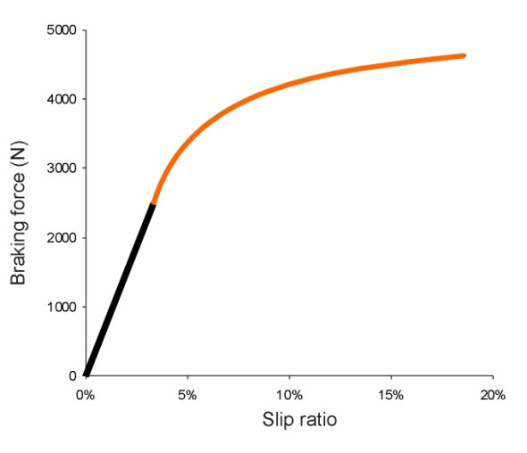
In figure 11, the braking force is plotted against slip ratio for a tyre with the same parameter values as the ones used earlier, except that the brush stiffness \(c\) is fixed a little higher at 4.5 MPa. The shape of the curve is similar (but not identical) to the earlier one for lateral force plotted against slip angle (figure 8). You can see how initially, the traction force increases with \(S\), but levels out as the slip zone extends further forward within the contact patch. Each increment of slip produces diminishing returns, and although it doesn’t appear within the range of values shown in the graph, when the slip ratio reaches unity the wheel locks and the braking force can rise no further.

Figure 11

Conclusion

Models of this kind explain broadly how the performance of a tyre - its ability to push the vehicle in the direction the driver wants to go - approaches a peak as the severity of the manoeuvre increases, and throw light on quirks of behaviour such as pneumatic trail. There is a caveat however. We’ve assumed that grip reaches a maximum and levels out thereafter, but in practice the available grip doesn’t level out but peaks and then falls as the tyre slides across the road surface, because the coefficient of sliding friction is less than the static value. This is one of the reasons why motor racing is more difficult than it looks: the driver is trying to achieve a delicate balance. If the car is pressed a fraction too hard some of the grip will vanish and the driver must do something quickly to regain it or risk disaster. This usually means losing momentum and losing time. On the other hand, if the car is not pressed hard enough, the driver still loses time. Fortunately perhaps, most of us don’t drive fast enough to use all the available grip, except when we encounter a road surface that is coated with ice, or a sheet of water that lifts the tyres clear of the road surface.