C.1603
The road surface
In the winter of 2009, about a million new potholes appeared on Britain’s roads. Potholes often draw complaints from the public, as do other bumps in the road that from time to time jolt the suspension and make car and bus travel uncomfortable. They include cobblestones, road surface repairs by utility companies, and the joints between concrete slabs on some post-war arterial roads. All of these irregularities occur on a scale of about 20 mm up to a metre across. But this is only a narrow band within a broader spectrum. If we step back from the road and view its profile over a length of several metres, we see that the surface undulates above and below the profile specified by the designer. Even when newly laid, the alignment is never perfect. The tolerance for a high-speed road is usually about +/- 6mm [22], and the UK standard specifies how often deviations of this order may occur within a road length of 300 m [19]. And on a larger scale, the road rises and falls by distances of several metres over local variations in ground level, and ultimately by several hundreds of metres over hills and valleys.
Road surface texture
There is roughness on a smaller scale too. In fact a perfectly smooth road surface would be dangerous to traffic, and roads are designed to present a particular kind of texture to vehicle tyres. At the coarser level, macro-texture occurs on a scale of 5 – 20 millimetres across [14] as shown in figure 1. On a smaller scale of the order of 0.5 millimetres across, there is micro-texture. In this section, we shall try to explain what these forms of texture looks like and how they provide grip between the wheel and the road.
Figure 1
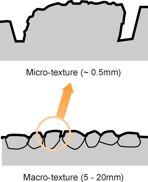
Macro-texture
Highway pavements are made, if you like, from stones and glue. There are two types of glue: the mixture of sand and cement that makes a concrete pavement rigid when it sets, and the rather more pliable bitumen used in asphalt and related materials (see Section C1602). The rest of the material consists of stone chippings usually referred to as ‘aggregate’: sharp-edged fragments usually obtained by crushing larger pieces of stone. Both concrete and bitumen roads are constructed in layers, and the surface layer provides the macro-texture that controls wet grip. When a pneumatic tyre rolls over a projecting asperity, the asperity dents the rubber and ploughs through it, putting energy into the tyre tread. Not all of this energy is given back, so there is a fall in contact pressure between the upstream side and the downstream side of the asperity. As explained in Section C1717, it is this asymmetry of pressures that provides hysteresis grip independently of whether the surface is wet or dry.
However, the effect of macro-texture depends on its shape as well as its size. The engineer wants depressions that are deep in short wavelengths (0.5 – 10mm) so that air can escape from the contact patch. Otherwise, sudden pressure changes will occur as air is trapped and then abruptly released: a major source of tyre noise. But at the same time, the depressions should be shallow in long wavelengths (10 – 50 mm), otherwise the tyre tread will rise and fall as it rolls over them, feeding vibrations into the suspension [26].
Figure 2
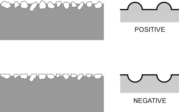
The profile can also be characterised in terms of ‘positive’ and ‘negative’ texture. At one extreme, we can imagine a perfectly level datum with chips or granules projecting above it (figure 2). This is referred to as ‘positive texture’, and it is typical of surface dressings, for example, which consist of stone chippings pressed onto a layer of molten bitumen that glues them to an existing pavement surface. At the other extreme, we can imagine a flat surface that is criss-crossed by indentations, so that each asperity has a flat top. This is referred to as ‘negative texture’. It is typical of porous asphalt, and it provides a running surface that is noticeably quieter for vehicle passengers and onlookers alike [20].
Microtexture
The term ‘microtexture’ refers to asperities measuring less than 0.5 mm across. It is the microtexture peaks that are responsible for adhesion, the kind of grip that we observe in friction experiments in the physics lab at school, and which provide the main contribution to tyre grip in dry weather. Microtexture also helps adhesion in wet weather, when a thin film of water is squeezed between the peak of each stone chipping and the tyre tread, forming a wedge that keeps the two surfaces apart (figure 3). The gritty surface associated with micro-texture can break through the film and restore adhesion on a lightly-wetted road surface [12].
Figure 3
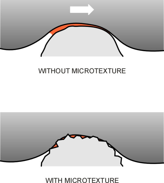
The degree of micro-texture varies from one type of aggregate to another, but all aggregates lose effectiveness over time as they become rounded by the scuffing of vehicle tyres. Stone chippings that project above the road surface tend to become polished and rounded with wear, which greatly reduces adhesion. There are two ways to delay this. The first is to use a soft material. Materials whose surface breaks away continually expose fresh micro-texture and therefore retain their skid resistance with wear. The second way is to use a hard material that is resistant to polishing. A local authority will often specify a proprietary anti-skid surfacing at a critical site such as the approach to a pedestrian crossing. The surfacing is quite thin, usually a single carpet of chippings embedded in a resin matrix and laid over a conventional surfacing material. The chippings are usually calcined bauxite, whose surface is gritty and resistant to abrasion. Chemically, it consists mostly of aluminium oxide (which in crystalline form is known as corundum) produced by heating bauxite-rich clay to a very high temperature.
Statistical modelling of the road surface profile
The springs on a road vehicle are meant to filter out the roughness injected by the road surface before it reaches the passenger cabin in the form of vibration. Manufacturers devote considerable time and effort to improving suspension performance in order to ensure their cars are smooth and quiet. Among other things, they try to predict the response of the vehicle to different kinds of road surface. If the road surface were to undulate in a regular fashion, the process would be relatively simple. One could simulate the effect on the vehicle by feeding a sine wave of the appropriate frequency into a simple mathematical model of the kind described in Section G1115 and predict the outcome directly. But as we have seen, the surface profile of a real road oscillates randomly above and below a notional datum line, with roughness on several different scales of measurement ranging from microscopic peaks and indentations in the surface material up to humps and troughs that stretch along several metres of carriageway. Fortunately, all of these inputs can be encapsulated in a single mathematical function.
Power spectral density curves
The solution is to represent the height of the road surface as a superposition of many simple curves: sine waves and cosine waves of different wavenumbers. The ‘wavenumber’ of any particular component is just the number of cycles per metre measured along the road, so for a signal of 2 cycles per metre, the wavelength will be 0.5 metres. A weak component (we shall call it a signal) has a small amplitude, meaning that the oscillation takes place over a narrow range above and below datum, less than a millimetre, say. A strong signal might have an amplitude of several millimetres, enough to shake the suspension of a car and make the ride uncomfortable.
The results can be pictured in the form of a power spectral density curve or PSD for short [6] [24]. It is derived from sample measurements of the road surface profile using a Fourier transform technique. High points along the curve indicate strong signals, while low points indicate weak ones. The term ‘power’ is a carry-over from electronic engineering, where it is common practice to measure the power content associated with different wavelengths rather than just the amplitude, and if the signal represents, for example, the voltage in an amplifier circuit, the power is proportional to the mean square of the voltage. Here, the signal represents road surface elevation, and the input is the height of the surface as it passes under the tyre, so the equivalent units are in square metres (m2). Finally, the curve measures the density of power output per unit waveband, so the equivalent power units are ‘square metres per cycle-per-metre’, or ‘m3cycle\(^{-1}\)’.
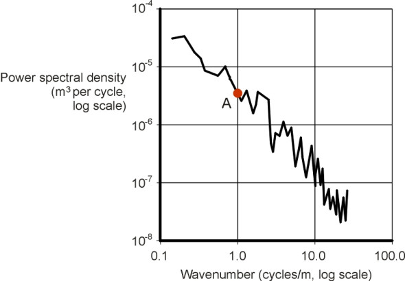
A notional PSD curve is shown in figure 4. It is plotted on a log-log scale because the wavenumbers and the PSD both vary over a wide range. The wavenumber is plotted along the horizontal axis, and the PSD value (mean square of the amplitude) corresponding to each wavenumber on the vertical axis. For example, the point ‘A’ on the curve in figure 4 corresponds to a wavenumber of 1 cycle m\(^{-1}\). The height of the curve at this point indicates a power spectral density of 4 \(\times\) 10\(^{-6}\) m3 cycle\(^{-1}\). The curve as a whole slopes downwards from left to right, so the PSD of the component waves starts high for small wavenumbers and decreases towards the right hand side of the graph as the wavenumber increases. This is what we would expect: for small wavenumbers which correspond to undulations several metres long, the road surface can rise or fall considerably so the waves have relatively high amplitudes. But at high wave numbers we are looking at individual stone chips projecting from the road surface, and the amplitude is relatively small. The graph terminates at a wavenumber of 100 cycles/m, because road surface irregularities smaller than 10 mm across don’t feed into a vehicle suspension in the same way as lower wavenumbers. The tyre contact patch bridges across them, and hence their impacts are largely absorbed by the tyre before they reach the springs.
Figure 4
Straight line approximations
During the late 1960s, surveyors began to sample the road surface profile in detail, recording the height at closely spaced intervals usually along the wheel tracks. More recently, it has been possible to extract profiles automatically using a mobile laser scanner mounted on a van. The amplitudes of the constituent signals can then be estimated through Fourier analysis of the digitised profile to yield a PSD curve. Examples of these curves can be found for example in [7] (derived from a vehicle test track at the UK Transport and Road Research Laboratory in 1973) and [10].
In each case, the PSD plot occupies a more-or-less straight band extending from top left to bottom right of the graph. Note that the band for a smooth road will appear lower down on the graph while the band for a rough one will appear further up. It is not difficult to fit a straight line to sample data of this kind, to generate a simple formula that can be fed into the simulation software used by manufacturers for analysing car and truck suspensions. Such a model can be found in [7], in our notation:
(1)
\[\begin{equation} N(\eta) \quad \sim \quad K \eta^{-2.5} \end{equation}\]where \(N(\eta)\) is the power spectral density in m3 per cycle, \(\eta\) is the wavenumber in cycles/m, and \(K\) is a constant coefficient in units of m\(^{0.5}\) cycles\(^{1.5}\). In the UK, \(K\) takes on values between 3 \(\times\) 10\(^{-8}\) and 50 \(\times\) 10\(^{-8}\) for a motorway, between 3 \(\times\) 10\(^{-8}\) and 800 \(\times\) 10\(^{-8}\) for a principal road, and between 50 \(\times\) 10\(^{-8}\) and 3000 \(\times\) 10\(^{-8}\) for a minor road [21]. A similar model appears in [11] and also in [1], which quotes values of the coefficients originally derived in 1973 [8].
The effect of vehicle speed
The waves described by equation 1 are frozen in concrete. But when you drive over them, the frequency \(f\) of the vibrations injected into your car’s suspension will vary according to how fast you are going. So there are two types of PSD: one to describe the spatial geometry of the road surface, and one to describe how the road surface varies over time as experienced by the wheels on your car. It’s the second kind that the vehicle designer is interested in. It quantifies the power density associated with any given frequency \(f\) and is denoted by \({F}(f)\).
Let the speed be \(V\) measured in m/s so that the distance you travel in one second is \(V\) metres. We want to know how a regular series of undulations of any given wavenumber translates into a signal acting on a vehicle tyre moving at that speed. Suppose the wavenumber is \(\eta\). The wheel of your car will encounter \(\eta V\) complete cycles of this particular road wave during every second, and will therefore experience a vibration of frequency \(\eta V\) hertz (a hertz is just one cycle per second), so
(2)
\[\begin{equation} f \quad = \quad \eta V \quad \end{equation}\]Conversely, if the wheel experiences a frequency \(f\), the vibration must come from road undulations of wavenumber \(\eta\) given by
(3)
\[\begin{equation} \eta \quad = \quad f/V \end{equation}\]But how strong will the signal be? Let’s look at wavenumbers in the short interval from \(\eta\) to \(\eta + \delta \eta\). Within this range, the PSD of the road surface elevation is \(N(\eta)\), and the power of the waves is equal to the area under the curve, which is \(N(\eta) \delta \eta{}\). Equation 2 tells us that a wheel running at speed \(V\) will experience the waves at the lower end \(\eta\) of this range as waves of frequency \(\eta V\) hertz, and waves at the upper end \(\eta + \delta \eta\) as waves of frequency \((\eta + \delta \eta)V\) hertz. The width of the interval is therefore transformed into \(V\delta \eta\) hertz. But the area under the PSD curve within this interval must be equal to the area under the original curve, which is \(N(\eta) \delta \eta\). Therefore the height of the curve (which equals the area divided by width) is \(N(\eta) \delta \eta / V \delta \eta\), which after cancelling the \(\delta \eta\) becomes \(N(\eta) / V\). It follows that when we translate the road surface PSD into a wheel input PSD, we must multiply the height of the original curve everywhere by the factor \(1/V\) thus:
(4)
\[\begin{equation} F(f) \quad = \quad N(\eta)/V \end{equation}\]and if we substitute for \(\eta\) using equation 3 we get
(5)
\[\begin{equation} F(f) \quad = \quad N(f/V)/V \end{equation}\]It is now possible to observe what happens to the strength of any particular signal frequency \(f\) when a car speeds up or slows down. Suppose the driver accelerates to a speed of \(2V\), i.e., twice the original speed. This affects the value of the PSD set out in equation 5 in two ways: first, the road waves that originally supplied the frequency under consideration are no longer relevant. The source of the vibration is now a road wave of twice the original length, i.e., the relevant wavenumber is halved. Since the wave-number graph slopes downwards from left to right, the signal will be stronger. Second, because the divisor term \(V\) on the right hand side of equation 5 is doubled, we must halve the result, which makes the signal weaker. It seems there are two opposing factors at work, so which has the greater influence? It turns out that for almost any conceivable road surface the slope of the ‘spatial’ PSD curve is sufficiently large to dominate, and the net effect is an increase in signal strength at the specified frequency.
A numerical example might help to make this clear, using the straight-line model set out in equation 1. Substituting the right-hand side for \(N(\eta)\) in equation 4 and replacing \(\eta\) by \(f/V\) we get:
(6)
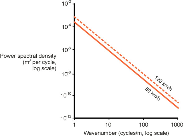
\[\begin{equation} F(f) \quad = \quad K f^{-2.5} V^{1.5} \end{equation}\]The equation is shown plotted as the solid curve in figure 5 for a car moving at 60 km/h on a road for which the value of the constant \(K\) is \(4\times 10^{-6}\). If the car now speeds up to 120 km/h, the value of \(F(f)\) in equation 6 is multiplied by a factor of 2\(^{1.5}\), and the curve shifts bodily upwards to a new position. We conclude that when we drive faster the road does indeed put more severe vibration into the suspension, and if equation 6 holds, this happens right across the frequency spectrum. In other cases, the overall magnitude of the increase will depend on the shape of the road PSD curve, and the change will not necessarily be uniform across all frequencies.
Figure 5
Skid resistance
The most important single feature of a road surface is the level of grip it provides for vehicle tyres. Elsewhere, we look at the mechanisms involved from the point of view of the tyre (Sections C0816 and C1717), but here, we shall concentrate on the road surface. Skid resistance is a term used by highway engineers to denote the coefficient of static friction on public roads. It varies markedly from place to place according to the age of the surface, the quality of the surface materials together with the quality of construction, and the weather. Table 1 shows some typical values for roads in the UK, culled from various sources. Ideally, one would expect a coefficient of about 1.0 on a dry road surface. Pedestrian walkways must have friction too, but not as much. Too much friction actually makes walking difficult [18].
| Road surface | Skid resistance |
| Dry | 0.8 - 1.0 |
| Wet | 0.2 - 0.65 |
| Icy | 0.05 - 0.10 |
Effect of surface water
If you compare them with what can be achieved with other materials, the figures in Table 1 are not particularly impressive. For example, the friction coefficient for rubber on a smooth glass sheet is much higher, around 1.6. But quite apart from the cost and practicality of using a material such as glass to support heavy lorries, a smooth surface only works when it is dry. As pointed out in a concise introduction to the subject by Woodside and Woodward [23], the real challenge is to design roads and tyres to cope with rain.
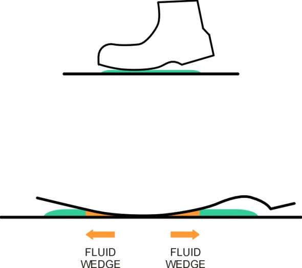
Water has a disastrous effect on friction. Imagine that someone has spilled a bottle of mineral water at your local supermarket, leaving a pool on the floor. You are pushing a trolley down the aisle towards the water. What happens next takes only a fraction of a second. When you step onto the liquid, the sole of your shoe compresses the film and pushes the water radially outwards. At first, the water can move out of the way quite easily, but as the gap narrows, it closes on a thin wedge of liquid. Water must be ejected faster and faster through a narrowing gap, and the thinner the gap, the more the pressure increases until it balances the pressure imposed by your foot (figure 6). You might just as well be skating on ice.
Figure 6
Fluid wedges turn up in other areas too, for example in the lubrication of plain bearings - see Section G1615 - and more spectacularly, when a ship’s hull slams downward into a wave trough. In the same way, as we saw earlier in figure 3, a fluid wedge can form on the top of a piece of stone aggregate projecting upward from the road surface as the tyre deforms around it. This is why neither roads nor tyres are constructed with smooth surfaces. Smooth surfaces are fine in dry weather, but the slightest rainfall or liquid spillage will result in a film that can lift the tyre away from the road. Hence the key to wet skid resistance is water dispersal. Here, we’ll consider the road surface only. The tyre is dealt with separately in Section C1610.
Dispersal of the water film
The road surface can be regarded as a container with a hole in the bottom. Water is poured in from above and drains away at a rate that depends on the level inside the container. The container is actually the whole carriageway surface, which is covered by a sheet of water moving steadily under the gravity down the steepest gradient until it leaves via a roadside drainage channel or sewer. In principle, the evolution of the film can be analysed mathematically or simulated on a computer.
The greatest risk from surface water arises on high-speed roads. High-speed roads tend to be wider than ordinary roads and therefore (a) they collect more rainwater per unit length, and (b) the rainwater has further to travel before it can find its way into a drain or gully. Together these factors imply a water film that is thicker than it would be on a narrow road, occasionally reaching a depth of several millimetres. In practice, roads are designed using empirical criteria recognising that the rate of dispersal depends on the length of the flow path, the slope along the flow path, and the road surface texture. More details can be found in [15] and [25]. The latter can be downloaded from the web site listed at the end of this section.
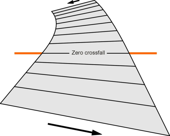
The most effective way to drain a road surface is to build in a lateral slope, usually not less than 2.5%. Two-way roads have a convex surface with a central crown, whereas most dual carriageways are constructed with two flat surfaces, each sloping towards the outside edge. But on curves, the slope of the outer carriageway is often reversed in order to provide superelevation, which reduces the lateral force on the vehicle tyres. Hence for the outer carriageway, water must drain towards the inside of the curve, and at some point along the transition between the entry to the curve and the curve itself, the lateral slope changes sign (figure 7). Since the surface cross-section is horizontal and dispersal is compromised, the designer will try to locate each of these critical points within an uphill or downhill section. A minimum longitudinal slope of 0.5% is a requirement in most countries.
Figure 7
Given the presence of water, how do the vehicle tyres and road surface deal with it? There are three main processes, each contributing directly or indirectly to wet grip [3]:
- Water is pumped away from the contact patch. This is done partly through grooves in the tyres, and partly through depressions in the road surface macro-texture, leaving a relatively thin film on each asperity peak.
- Road surface micro-texture penetrates the remaining water film to create adhesion,
- The rubber tyre tread generates grip through hysteresis.
Nevertheless, water on a road surface will usually reduce tyre grip by a half, and more in a heavy rainstorm. The worst case occurs when the surface of the water film rises above the asperity peaks to form a continuous sheet.
Aqua-planing
Vehicle tyres rely on their grooving pattern to displace the water so that the blocks in between make good contact with the road surface. Effectively, the tread acts as a pump, and the rate at which it is required to displace water increases with both speed and water depth. The water isn’t displaced immediately, and the relationship between the tyre and the road can be broken down into three separate phases within the contact patch [13]. At the leading edge of the contact patch, surface water builds up into a wedge. Further aft, some of the water is displaced so that macro-texture peaks can develop contact or partial contact with the tread blocks. At the rear of the contact patch, the film is sufficiently thin for micro-texture peaks to penetrate.
The influence of speed is crucial. As speed increases, pressure builds up within the leading wedge, which extends rearwards. At still higher speeds, the boundaries separating the three zones move rearwards until the tread lifts clear of the road surface: a phenomenon known as aqua-planing (figure 8). Given sufficient vehicle speed, aqua-planing starts when the film thickness reaches about 2.5 mm [16], and when it reaches 4 mm the tyres lose their grip and the driver has no control over steering. A detailed analysis of the process can be found in [5].
Figure 8

Porous asphalt
The risk of aqua-planing can be reduced if the road surfacing material lets rainwater percolate into the road surface as well as across it. This is one of the properties of porous asphalt, whose interconnecting voids occupy some 20% of the total volume [4]. But although it can cope with moderate levels of rainfall, when its capacity is reached the water will overflow and the asphalt behaves like a non-porous surface [25].
Figure 9
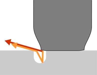
Porous asphalt also reduces noise. The mechanism relies on ‘destructive interference’: peaks in the sound pressure waves are matched against the troughs associated with the same signal so that the two cancel each other out. Here, the noise source is the tyre contact patch, which creates bursts of high pressure as successive blocks strike the road surface. Some of the resulting noise energy is propagated away from the contact area, travelling above the road surface directly to the observing standing by the roadside. The remaining noise energy enters pores in the road surface and is reflected, reaching the observer by a slightly longer route. Because they are out of phase, some waves will cancel each other out and the overall noise is reduced (figure 9). In addition to reducing tyre noise, the pores also absorb some of the vehicle engine noise that would otherwise be reflected from the road surface, and reduce the glare from headlamps at night. However, porous asphalt must be reinforced with fibres or polymer additives to withstand heavy wheel loads. Alternative non-porous wearing course systems are now available that perform nearly as well.