A simple model

In practice, a suspension consists of many elements that interact in a complex way so that the wheel can move up and down relative to the vehicle body. The spring provides most but not all of the flexibility: all the component parts deform under load to a certain degree, especially the pneumatic tyre. For example, a tyre tread surrounds local irregularities in the road surface such as the sharp edge of a pothole or coarse particles of aggregate projecting from an asphalt road surface. Both would otherwise inject high-frequency disturbances into the vehicle. Hence the tyre filters out frequencies that are too high for the main spring and damper system to deal with efficiently, usually in the range 20 – 400Hz [2].

There are other elements in the suspension linkage such as rubber bushes at the hinges that provide additional compliance and affect the transmission of high frequency vibrations. Hence it is usual to picture the suspension as a ‘cascade’ of springs and dampers that modify the vibrations imparted by the track running surface before they reach the passenger compartment. Each additional spring introduces an extra degree of freedom in the sense that relative movement can take place independently at each stage. If all these are taken into account, modelling of suspension becomes very complicated so suspension designers use computer simulation software to handle the calculations.

However, in the case of a motor car, the principles can be illustrated with a two degrees-of-freedom model with the tyre at the first tier and the spring-and-damper at the second, or even a single degree-of-freedom model with spring and damper only. In either case we ignore the flexibility of the other components altogether. To start with, we must explain two of the parameters that characterise suspension behaviour.

Figure 1

Static deflection

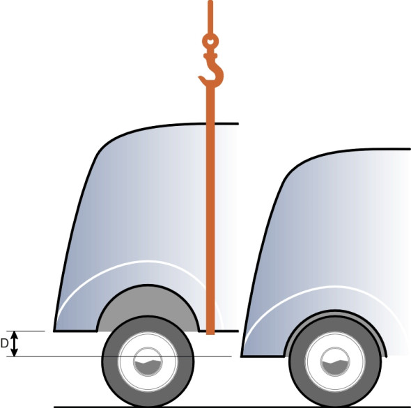
Imagine a car hanging from a crane with its wheels just touching the ground (figure 1). It is lowered gradually until it settles into its equilibrium position. For any given wheel, the static deflection\(\; D\) is the distance moved upwards by the wheel relative to the body when it settles [9]. If the load-deflection curve of the spring is a straight line, its stiffness \(k\) is equal to the slope (see Section G1114), so that

where \(P\) is the load carried by the wheel in question. As will be explained in a moment, for a saloon car an ideal value for the static deflection is about 250 mm (10 inches), but most cars have less, with small cars around half that much [4]. This information, together with the static wheel load \(P\), essentially fixes the suspension stiffness regardless of any other requirements.

Natural frequency

Another important characteristic of a suspension system for any given wheel is the natural frequency\(\; f_N\), the frequency at which it will oscillate after receiving a single jolt. In fact there are several natural frequencies, each associated with a different ‘spring’ in the cascade, but here we are interested in the one associated with the main suspension spring. Let’s assume it has linear properties and ignore the effect of the damper and the tyre (neither have much effect on \(N\)). And let’s treat the suspension spring together with the part of the vehicle it supports as an isolated system. Then as shown in the Appendix, the value of \(f_N\) is given by the formula

in units of hertz, i.e., cycles per second. This relationship shows how the load on the wheel affects the ‘softness’ of the ride: if \(P\) doubles, the natural frequency decreases by a factor of \(\sqrt 2\), and therefore the heavier the load, the slower the bounce. A heavily-loaded car may not be very safe, but it gives a smoother ride.

equation 2 can be expressed in a slightly different way by substituting \(D\) for \(P/k\):

As we saw earlier in the rubber band experiment in Section G1114, to minimise bouncing of the car body, the natural frequency should be as far as possible below the frequency of any waves or bumps in the surface. Ideally this means around 1 Hz, from which we deduce via equation 3 that the static deflection needs to be of the order of 250 mm.

The quarter-car model

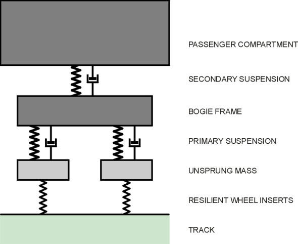
We’ve simplified the suspension model by ignoring any flexibility in the links and bushes, and in order to work out the natural frequency, we treated a single wheel supporting one corner of the car as if its behaviour could be considered in isolation from the rest of the vehicle. Such a ‘quarter car’ model is shown diagrammatically in figure 2, where the two zig-zag lines represent elastic springs (one is the tyre and the other is the suspension spring proper). The piston-and-cylinder on the right-hand side represents a damper. In practice, of course, an automobile body responds simultaneously to roughness input through all four wheels, and the four suspension springs to some extent interact. But before computers became widely available, the quarter-car model provided a useful indication of how a suspension was likely to perform, and it is still used for purposes of illustration [1] [3] [6]. Unfortunately, rail vehicles can’t be dealt with in this way because although the same general principles apply, passenger coaches (and many freight vehicles nowadays) carry two separate suspension systems, one stacked on top of the other. The cascade is hierarchical, with input from the primary suspension associated with each of 2 axles of a bogie feeding into the secondary system (figure 3).

Figure 2

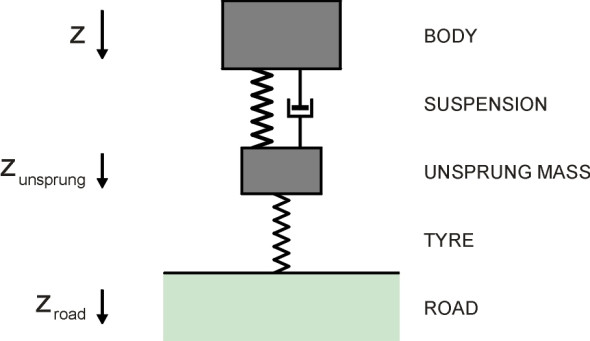
Figure 3

Suspension performance

We are now in a position to model the process mathematically, with damping included. Our model framework is the single degree-of-freedom quarter-car model as shown in figure 2 but with the tyre ‘spring’ removed; we now have just one spring and one damper in parallel. Since the tyre is not included, the model doesn’t take into account ‘wheelhop’ vibrations associated with the unsprung mass. Results for the case where a second ‘spring’ represents the tyre can be found in [5]. And we shall measure output as vibration delivered not to the passenger’s torso, but to the vehicle body at the suspension mounting points, which is not quite the same thing. Nevertheless, the results show broadly how to manipulate the properties of the spring and damper to improve the quality of the ride.

Figure 4

Free oscillations

Imagine the system freely oscillating after an initial disturbance (someone presses down on the bodywork and then lets go). Vertical displacements of the body are denoted by z, measured positive downwards relative to the equlibrium position at rest (static deflection). The mass of the quarter-body is \(M\), the spring stiffness \(k\), and the damping coefficient \(c\). We picture the body at displacement \(z\) after time \(t\), and work out all the forces acting on it as follows:

1. Weight: the weight of the quarter-body can be pictured as a force \(Mg\) acting vertically downward at the axle centreline.
2. Spring force: since the spring deflection is \(D + z\), the spring force (measured at the wheel) is equal to stiffness times deflection or \(- k(D + z)\). It is negative because it acts upwards on the quarter-body.
3. Damper force: the damper exerts a force equal to the damping coefficient times speed, in other words \(-c\frac{dz}{dt}\). It acts in the opposite direction to the motion, and again its sign is negative.

The sum of these forces is \(Mg - k(D + z) - c\frac{dz}{dt}\). Since \(\textit{force} = \textit{mass} \times \textit{acceleration}\), we can write down the equation of motion for the quarter-body as

But at static equilibrium, we know from equation 1 that \(kD = \textit{applied load} = Mg\), so the first and last terms on the right-hand side cancel leaving

which can be re-written

This is a second-order linear differential equation with constant coefficients, and its general solution is (see for example [8]):

where \(B_1\) and \(B_2\) are arbitrary constants whose values depend on the initial conditions, and \(m_1\) and \(m_2\) are the roots of the characteristic equation

To simplify matters later on, mathematicians like to replace the original coefficients \(c/M\) and \(k/M\) with new ones \(\omega\) and \(\zeta\) (the lower-case Greek letters omega and zeta), thus:

and

which transforms the characteristic equation into

The solutions to the characteristic equation depend on the value of \(\zeta\):

where \(j\) is the square root of minus one. It may now become clear why we switched coefficients. The quantity \(\omega\) is just the natural frequency, which we have already met expressed in different units. To see this, replace the wheel load \(P\) in equation 2 by \(Mg\), square both sides and swap them around to get

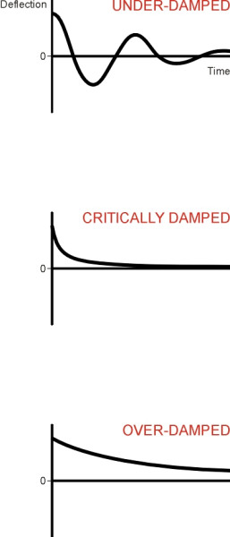
From this we see that \(\omega = 2 \pi f_N\), and it is measured in radians per second. The dimensionless quantity \(\zeta\) symbolised by the Greek letter ‘zeta’ is known as the damping parameter. Because the damper exerts a force that continually dissipates energy, the system must decay towards its static equilibrium position, and the value of \(\zeta\) determines the manner in which this happens. When its value is less than one, the system is said to be under-damped. The car body will oscillate indefinitely, but with decreasing amplitude (figure 4). When its value is greater than one, the damper resists movement to such a degree that it prevents the body from ever reaching the equilibrium position. When its value is equal to one, the car body is said to be critically damped. It decays more rapidly than in either of the two preceding cases, but will not quite oscillate. All cars are under-damped, with the damping parameter \(\zeta\)typically fixed at around 0.4.

Figure 5

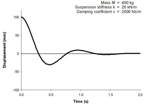
figure 5 shows a specific response curve for a quarter-vehicle of mass 400 kg having a spring stiffness of 20 kN/m and damping coefficient 2000 Ns/m. It was obtained by calculating the parameters \(\omega\) and \(\zeta\) via equation 9 and equation 10, which came to 7.07 rad/s and 0.35 respectively. Substitution of these values into equation 11 yielded roots \(m_1\) and \(m_2\) that in turn were substituted into equation 7 to re-create the time profile of body motion from a starting position 100 mm below static equilibrium. The resulting curve shows that the body returns to its equilibrium position quite quickly. There is no prolonged bouncing up and down. You can confirm this by leaning on a car and letting go.

Forced oscillations

So far, we have pictured the vehicle standing still, vibrating only as the result of a single impulse or blow to the body. But when moving along the road, it receives a continuous input of vibration from the wheels. The vibration is a mixture of frequencies representing the irregularities that make up the road surface profile, all of which feed into the wheels simultaneously. Denote the height of the road surface at any point relative to its mean datum by \(z_{road}\). The wheel is assumed to move up and down as it traces out the fluctuations in \(z_{road}\). These wheel motions form the input. They are transmitted through the suspension to the vehicle body whose motion constitutes the output, with different frequencies attenuated to a greater or lesser degree by the spring and damper combination. In principle, the effects can be analysed using computer simulation coupled with a statistical representation of the road surface, whose general form is sketched out in section C1603. But in order to see which frequencies are likely to cause problems, we can calculate the response separately for each frequency of interest and plot the results on a graph.

To generate any given input frequency, the surface profile of the road is pictured as a regular sine wave with peaks rising a distance \(a\) metres above the mean and troughs \(a\) metres below, that is to say, the input amplitude is \(a\). If the wavelength is \(L\), a vehicle moving at speed \(V\) will encounter a peak every \(L/V\) seconds, and the frequency is therefore \(V/L\) cycles per second (hertz). Put \(\Omega = 2 \pi V/L\). Then the wheel will oscillate with a vertical displacement given by

The only change compared with the scenario described in the last section is the nature of the input. Here, the wheel is forced to move up and down by a specified amount, which alters the deflection of the spring and damper. The two terms on the right-hand side of equation 5 are therefore modified. The deflection of the spring becomes \(z - a\sin(\Omega t)\), and the speed of damper compression becomes

The new equation of motion is

which can be rearranged in the form

The solution consists of two parts: the ‘particular integral’ and the ‘complementary function’. The complementary function is the same as for equation 6, but it doesn’t concern us here, because it decays to zero over time. We are interested in the way the vehicle bounces when driven steadily over a road with continuous vibration input. Hence we need the particular integral, which takes the form:

where \(C_1\) and \(C_2\) are arbitrary constants. This solution can be substituted back into equation 17, and by equating terms in \(\sin (\Omega t)\) and then terms in \(\cos (\Omega t)\), one can solve for \(C_1\) and \(C_2\) and finally show that the amplitude \(A(\Omega)\) of the response, equal to \(\sqrt {{C_1}^2 \; + \; {C_2}^2}\), is given by

What does all this amount to? If there are waves in the road surface, the wheel moves up and down with the waves. It passes on the motion to the spring-and-damper system, which in turn passes it on to the body but in modified form. The result is vehicle body vibration: the quarter-body moves up and down echoing the movements of the wheels, but not necessarily in phase or by the same amount. Hence if the road surface input is a regular sine wave of amplitude \(a\) metres at a frequency of \(\Omega\) rad/s, the quarter-body oscillates at the same frequency but with a different amplitude whose value depends on \(\Omega\).

Figure 6

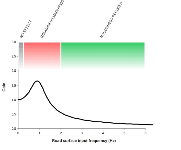
The ratio \(A(\Omega)/a\) of the two amplitudes is sometimes called gain by analogy with amplification in electrical circuits (see, for example, [3]). By calculating the gain we can see how the suspension has damped or amplified the waves. The results for our single-degree-of-freedom model are shown in figure 6 for a suspension with a damping parameter \(\zeta\) equal to 0.4, and natural frequency \(\omega\) equal to 6.28 rad/s (1 Hz). What do we expect to find? At very low frequencies, we expect the body to copy the wheel motion exactly. When the wheel climbs up a hill and rolls down the other side, the body climbs with it, tracing out an identical path. Therefore, input and output are equal and the gain is 1.0. But as the frequency increases, the gain increases too, because when the wheel rises over a more localised undulation, the body ‘bounces’ on its springs. Effectively, undulations in the road such as a hump-backed bridge are magnified. As you might expect, the gain is largest around the natural frequency, and this is critical for road construction. It’s important to avoid waves in the road surface that inject pulses at frequencies around 1 Hz. But for frequencies above 1.5 Hz, the suspension cuts down the level of vibration appreciably, which is what we want. For example, for a road surface that injects sinusoidal waves at a frequency of 5 Hz, the gain is about 0.16. So if the road surface waves have an amplitude of 10 mm, the body vibration will have an amplitude of about 0.16 \(\times\) 10 mm, or 1.6 mm. There is a six-fold reduction in the disturbances that get through to the passenger compartment.

Figure 7

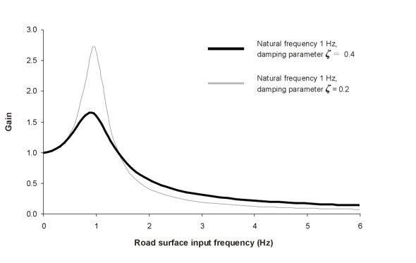
How does the picture change if we alter the suspension characteristics? Can the results be improved? In figure 7, the second, grey curve represents what happens if the damping is halved. Performance at the higher frequencies is improved, but at a price. Close to the natural frequency, the gain nearly doubles. The low-frequency bumps and waves will become much more noticeable for passengers. In a similar way, one can work out what happens if the damping is made more robust. The curve isn’t plotted in figure 7, but as you can guess, the opposite effect occurs. The body does not bounce so energetically at the natural frequency, but high-freqency response gets worse. One might describe this suspension set-up as ‘hard’.

Phase lag and energy losses

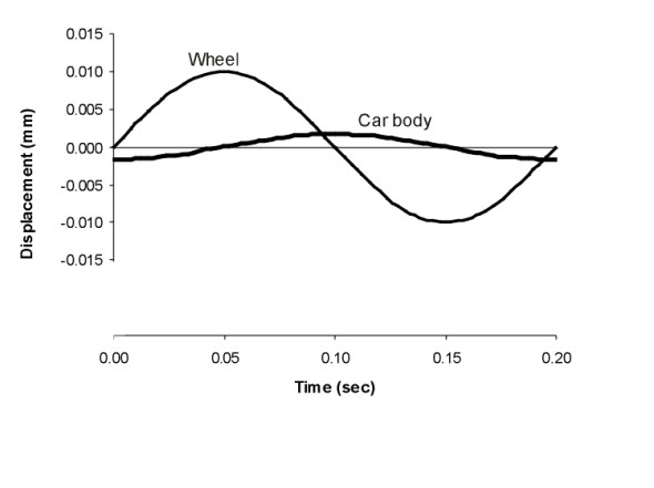
Now for the final step. We have seen that when the wheels bounce up and down, the body bounces up and down too, but mostly to a lesser extent. A characteristic feature of this motion is that the wheels and body don’t move in the same direction at the same time. Their motions are out of phase as shown in figure 8: there is a time lag between deflection of the wheel and deflection of the body. To understand the consequences, it helps to focus on what is going on inside the suspension. How does the spring-damper combination respond when it is squeezed and extended?

Figure 8

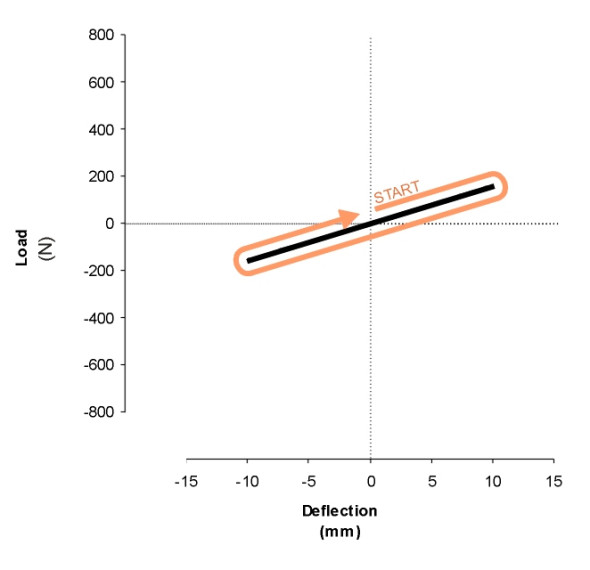
Industrial products are often tested in the laboratory to see how they respond to loading. For example, a steel spring may be clamped in a testing machine and subjected to a tensile load. It will elongate roughly in proportion to the applied load, with the values of load and deformation tracing out a curve such as the grey line shown in figure 9, where tension is taken as positive so the trajectory starts off towards the right-hand side of the graph. The load is then removed, and provided the relaxation is gradual, the load and deformation will trace out the same curve in reverse. The spring can now be compressed, with the load increasing to maximum and then being gradually removed. Again, the values of load and deformation will trace out a single curve, this time in the negative region.

Figure 9

But when they are loaded and unloaded very quickly, not all objects behave in this way, and nor does a vehicle suspension unit. We can illustrate this using the quarter-vehicle model with suspension parameter values equal to the ones used in the previous example (\(\zeta =\) 0.4 and \(\omega =\) 6.28 rad/s, with a sinusoidal road surface input of amplitude 10 mm at a frequency of 5 Hz). Our model is not a very realistic one because a real damper doesn’t behave in the idealised way we have have assumed here (see for example [10]), but nevertheless the results are interesting.

Figure 10

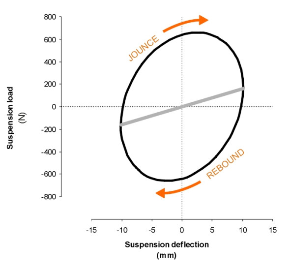
In figure 10, deflections are plotted along the horizontal axis, and forces on the vertical axis. The grey line represents the load-deflection curve under gradual or static loading, and is similar to the one shown in figure 9. By contrast, the black curve represents the ‘dynamic’ behaviour with a rapidly oscillating input. During the compression stroke, successive points trace a path up the left-hand side of the ellipse, while during the rebound stroke the path returns down the right-hand side. The two paths are different. Since the area under any segment of the curve is equal to force times distance moved, each segment can be interpreted as an energy flow: the jounce stroke puts energy into the suspension, and the rebound stroke takes it out. But the two are not equal, and the area enclosed within the ellipse represents energy lost to the system; in fact it appears as heat in the damper fluid and is eventually lost to the atmosphere. The heat energy dissipated by damping is an example of hysteresis. In the present example, it comes to around 100 watts, about the same as an old-fashioned tungsten domestic light bulb.

Appendix: Simple harmonic motion of a mass supported by a spring

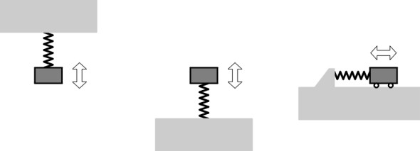
If you suspend a mass \(M\) from an idealised spring the mass will undergo ‘simple harmonic motion’, oscillating up and down at a certain characteristic frequency, rather like a pendulum. ‘Idealised’ means that the spring is linear and neither the mass nor the spring are affected by friction or damping. The same applies to a mass sitting on top of the spring, or being pushed and pulled from side to side as shown in figure 11. Looking at the middle diagram, let us imagine first removing mass and then lowering it onto the spring. If we allow it to settle to its equilibrium position, the spring will deflect by an amount

(20)

\[\begin{equation} D \quad = \quad \frac{mg}{k} \end{equation}\]

We’ll measure any subsequent vertical displacement \(z\) of the mass relative to the equilibrium position, positive downwards. At displacement \(z\), the compression force in the spring is equal to \(k(D+z)\), which if we substitute for \(D\) via equation 20comes to \(Mg+kz\). The total downwards force acting on the body is equal to its weight minus the upwards thrust \(Mg+kz\) from the spring thus:

(21)

\[\begin{equation} Mg \; - \; (Mg\,+\,kz) \quad = \quad -kz \end{equation}\]

Since force equals mass times acceleration we can then write the equation of motion of the mass as

(22)

\[\begin{equation} M \frac{d^{2}z}{dt^2} \quad = \quad -kz \end{equation}\]

which leads to a second-order linear differential equation whose solution (see, for example, [7]) is a sine wave of frequency \(f_N\) given by

(23)

\[\begin{equation} f_N \quad = \quad \frac{1}{2 \pi} \sqrt{\frac{k}{M}} \quad \text{Hz} \end{equation}\]

For a vehicle suspension at a wheel that carries a static load \(P\), we can substitute \(P/g\) for the mass \(M\) in the above equation and predict the natural frequency of the suspension as

(24)

\[\begin{equation} f_N \quad = \quad \frac{1}{2 \pi} \sqrt{\frac{kg}{P}} \quad \text{Hz} \end{equation}\]

Revised 11 February 2015

Figure 11